In the real world we cannot know all the positions, velocities and forces exactly, but the corollary to Laplace’s belief was that if we knew approximate values at one instant, the universe would not be much different anyway. This was reasonable, for surely sprinters who started a tenth of a second after the gun had fired would break the tape only a tenth of a second off their usual time. The belief was that small discrepancies in initial conditions meant small discrepancies in outcomes. Chaos theory exploded this idea.

The butterfly effect

The butterfly effect shows how initial conditions slightly different from the given ones, can produce an actual result very different from the predictions. If fine weather is predicted for a day in Europe, but a butterfly flaps its wings in South America then this could actually presage storms on the other side of the world – because the flapping of the wings changes the air pressure very slightly causing a weather pattern completely different from the one originally forecast.

We can illustrate the idea with a simple mechanical experiment. If you drop a ball-bearing through the opening in the top of a pinboard box it will progress downwards, being deflected one way or the other by the different pins it encounters on route until it reaches a finishing slot at the bottom. You might then attempt to let another identical ball-bearing go from the very same position with exactly the same velocity. If you could do this exactly then the Marquis de Laplace would be correct and the path followed by the ball would be exactly the same. If the first ball dropped into the third slot from the right, then so would the second ball.

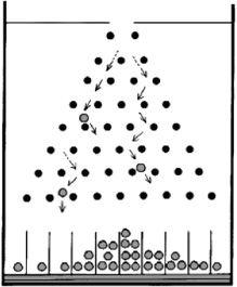
Pinboard box experiment

But of course you cannot let the ball go from exactly the same position with exactly the same velocity and force. In reality, there will be a very slight difference which you might not even be able to measure. The result is the ball-bearing may take a very different route to the bottom and probably end up in a different slot.

A simple pendulum

The free pendulum is one of the simplest mechanical systems to analyse. As the pendulum swings back and forth, it gradually loses energy. The displacement from the vertical and the (angular) velocity of the bob decrease until it is eventually stationary.

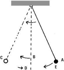
The free pendulum

The movement of the bob can be plotted in a phase diagram. On the horizontal axis the (angular) displacement is measured and on the vertical axis the velocity is measured. The point of release is plotted at the point A on the positive horizontal axis. At A the displacement is at a maximum and the velocity is zero. As the bob moves through the vertical axis (where the displacement is zero) the velocity is at a maximum, and this is plotted on the phase diagram at B. At C when the bob is at the other extremity of its swing, the displacement is negative and the velocity is zero. The bob then swings back through D (where it is moving in the opposite direction so its velocity is negative) and completes one swing at E. In the phase diagram this is represented by a rotation through 360 degrees, but because the swing is reduced the point E is shown inside A. As the pendulum swings less and less this phase portrait spirals into the origin until eventually the pendulum comes to rest.

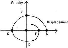
Phase diagram for the simple pendulum

This is not the case for the double pendulum in which the bob is at the end of a jointed pair of rods. If the displacement is small the motion of the double pendulum is similar to the simple pendulum, but if the displacement is large the bob swings, rotates, and lurches about and the displacement about the intermediate joint is seemingly random. If the motion is not forced, the bob will also come to rest but the curve that describes its motion is far from the well-behaved spiral of the single pendulum.

Chaotic motion

The characteristic of chaos is that a deterministic system may appear to generate random behaviour. Let’s look at another example, the repeating, or iterative, formula a × p × (1 – p) where p stands for the population, measured as a proportion on a scale from 0 to 1. The value of a must be somewhere between 0 and 4 to guarantee that the value of p stays in the range from 0 to 1.

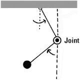
Movement of double pendulum

Let’s model the population when a = 2. If we pick a starting value of, say p = 0.3 at time = 0, then to find the population at time = 1, we feed p = 0.3 into a × p × (1 – p) to give 0.42. Using only a handheld calculator we can repeat this operation, this time with p = 0.42, to give us the next figure (0.4872). Progressing in this way, we find the population at later times. In this case, the population quickly settles down to p = 0.5. This settling down always takes place for values of a less than 3.

If we now choose a = 3.9, a value near the maximum permissible, and use the same initial population p = 0.3 the population does not settle down but oscillates wildly. This is because the value of a is in the ‘chaotic region’, that is, a is a number greater than 3.57. Moreover, if we choose a different initial population, p = 0.29, a value close to 0.3, the population growth shadows the previous growth pattern for the first few steps but then starts to diverge from it completely. This is the behaviour experienced by Edward Lorenz in 1961 (see box).

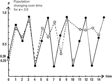
Population changing over time for a = 3.9

Forecasting the weather

Even with very powerful computers we all know that we cannot forecast the weather more than a few days in advance. Over just a few days forecasting the weather still gives us nasty surprises. This is because the equations which govern the weather are nonlinear – they involve the variables multiplied together, not just the variables themselves.

From meteorology to mathematics

The discovery of the butterfly effect happened by chance around 1961. When meteorologist Edward Lorenz at MIT went to have a cup of coffee and left his ancient computer plotting away he came back to something unexpected. He had been aiming to recapture some interesting weather plots but found the new graph unrecognizable. This was strange for he had entered in the same initial values and the same picture should have been drawn out. Was it time to trade in his old computer and get something more reliable?

After some thought he did spot a difference in the way he had entered the initial values: before he had used six decimal places but on the rerun he only bothered with three. To explain the disparity he coined the term ‘butterfly effect’. After this discovery his intellectual interests migrated to mathematics.

The theory behind the mathematics of weather forecasting was worked out independently by the French engineer Claude Navier in 1821 and the British mathematical physicist George Gabriel Stokes in 1845. The Navier–Stokes equations that resulted are of intense interest to scientists. The Clay Mathematics Institute in Cambridge, Massachusetts has offered a million dollar prize to whoever makes substantial progress towards a mathematical theory that unlocks their secrets. Applied to the problem of fluid flow, much is known about the steady movements of the upper atmosphere. But air flow near the surface of the Earth creates turbulence and chaos results, with the subsequent behaviour largely unknown.

While a lot is known about the theory of linear systems of equations, the Navier–Stokes equations contain nonlinear terms which make them intractable. Practically the only way of solving them is to do so numerically by using powerful computers.

Strange attractors

Dynamic systems can be thought of possessing ‘attractors’ in their phase diagrams. In the case of the simple pendulum the attractor is the single point at the origin that the motion is directed towards. With the double pendulum it’s more complicated, but even here the phase portrait will display some regularity and be attracted to a set of points in the phase diagram. For systems like this the set of points may form a fractal  which is called a ‘strange’ attractor that will have a definite mathematical structure. So all is not lost. In the new chaos theory, it is not so much ‘chaotic’ chaos that results as ‘regular’ chaos.

the condensed idea

The wildness of regularity