There is interesting problem in which the idea of probability is required. It is the problem of the “random walk.” In its simplest version, we imagine a “game” in which a “player” starts at the point x=0 and at each “move” is required to take a step either forward (toward +x) or backward (toward −x). The choice is to be made randomly, determined, for example, by the toss of a coin. How shall we describe the resulting motion? In its general form the problem is related to the motion of atoms (or other particles) in a gas—called Brownian motion—and also to the combination of errors in measurements. You will see that the random-walk problem is closely related to the coin-tossing problem we have already discussed.

First, let us look at a few examples of a random walk. We may characterize the walker’s progress by the net distance D_N traveled in N steps. We show in the graph of Fig. 6–5 three examples of the path of a random walker. (We have used for the random sequence of choices the results of the coin tosses shown in Fig. 6–1.)

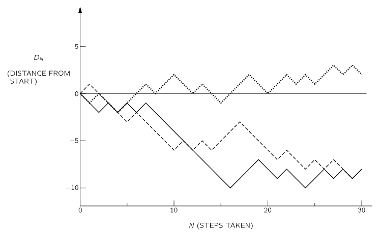
Fig. 6–5. The progress made in a random walk. The horizontal coordinate N is the total number of steps taken; the vertical coordinate D_N is the net distance moved from the starting position.

What can we say about such a motion? We might first ask: “How far does he get on the average?” We must expect that his average progress will be zero, since he is equally likely to go either forward or backward. But we have the feeling that as N increases, he is more likely to have strayed farther from the starting point. We might, therefore, ask what is his average distance travelled in absolute value, that is, what is the average of |D|. It is, however, more convenient to deal with another measure of “progress,” the square of the distance: D² is positive for either positive or negative motion, and is therefore a reasonable measure of such random wandering.

We can show that the expected value of D²_N is just N, the number of steps taken. By “expected value” we mean the probable value (our best guess), which we can think of as the expected average behavior in many repeated sequences. We represent such an expected value by ⟨D²_N⟩, and may refer to it also as the “mean square distance.” After one step, D2 is always +1, so we have certainly ⟨D²₁⟩=1. (All distances will be measured in terms of a unit of one step. We shall not continue to write the units of distance.)

The expected value of D²_N for N>1 can be obtained from D_N−1. If, after (N−1) steps, we have D_N−1, then after N steps we have D_N=D_N−1+1 or D_N=D_N−1−1. For the squares,

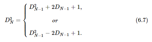
In a number of independent sequences, we expect to obtain each value one-half of the time, so our average expectation is just the average of the two possible values. The expected value of D²N is then D²_N−1+1. In general, we should expect for D²_N−1 its “expected value” ⟨D²_N−1⟩ (by definition!).

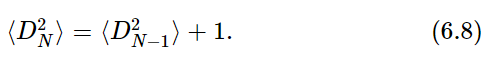
We have already shown that ⟨D²₁⟩=1; it follows then that

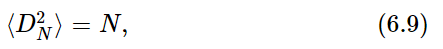
a particularly simple result!

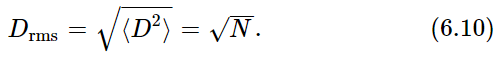
If we wish a number like a distance, rather than a distance squared, to represent the “progress made away from the origin” in a random walk, we can use the “root-mean-square distance” D_rms:

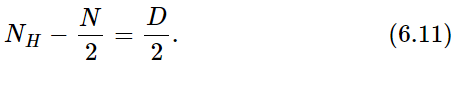
We have pointed out that the random walk is closely similar in its mathematics to the coin-tossing game we considered at the beginning of the chapter. If we imagine the direction of each step to be in correspondence with the appearance of heads or tails in a coin toss, then D is just N_H−N_T, the difference in the number of heads and tails. Since N_H+N_T=N, the total number of steps (and tosses), we have D=2N_H−N. We have derived earlier an expression for the expected distribution of N_H (also called k) and obtained the result of Eq. (6.5). Since N is just a constant, we have the corresponding distribution for D. (Since for every head more than N/2 there is a tail “missing,” we have the factor of 2 between N_H and D.) The graph of Fig. 6–2 represents the distribution of distances we might get in 30 random steps (where k=15 is to be read D=0; k=16, D=2; etc.).

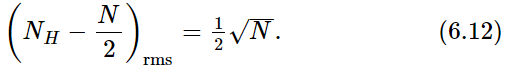
The variation of N_H from its expected value N/2 is

The rms deviation is

According to our result for D_rms, we expect that the “typical” distance in 30 steps ought to be √30≈5.5, or a typical k should be about 5.5/2=2.75 units from 15. We see that the “width” of the curve in Fig. 6–2, measured from the center, is just about 3 units, in agreement with this result.

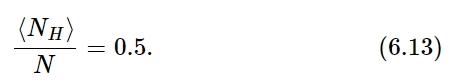
We are now in a position to consider a question we have avoided until now. How shall we tell whether a coin is “honest” or “loaded”? We can give now at least a partial answer. For an honest coin, we expect the fraction of the times heads appears to be 0.5, that is,

We also expect an actual N_H to deviate from N/2 by about √N/2, or the fraction to deviate by

The larger N is, the closer we expect the fraction N_H/N to be to one-half.

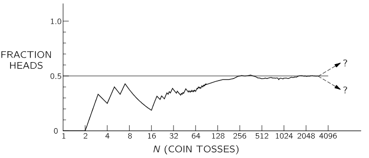
Fig. 6–6. The fraction of the tosses that gave heads in a particular sequence of N tosses of a penny.

In Fig. 6–6 we have plotted the fraction N_H/N for the coin tosses reported earlier in this chapter. We see the tendency for the fraction of heads to approach 0.5 for large N. Unfortunately, for any given run or combination of runs there is no guarantee that the observed deviation will be even near the expected deviation. There is always the finite chance that a large fluctuation—a long string of heads or tails—will give an arbitrarily large deviation. All we can say is that if the deviation is near the expected 1/2√N (say within a factor of 2 or 3), we have no reason to suspect the honesty of the coin. If it is much larger, we may be suspicious, but cannot prove, that the coin is loaded (or that the tosser is clever!).

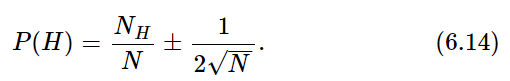
We have also not considered how we should treat the case of a “coin” or some similar “chancy” object (say a stone that always lands in either of two positions) that we have good reason to believe should have a different probability for heads and tails. We have defined P(H)=⟨N_H⟩/N. How shall we know what to expect for N_H? In some cases, the best we can do is to observe the number of heads obtained in large numbers of tosses. For want of anything better, we must set ⟨N_H⟩=N_H(observed). (How could we expect anything else?) We must understand, however, that in such a case a different experiment, or a different observer, might conclude that P(H) was different. We would expect, however, that the various answers should agree within the deviation 1/2√N [if P(H) is near one-half]. An experimental physicist usually says that an “experimentally determined” probability has an “error,” and writes

There is an implication in such an expression that there is a “true” or “correct” probability which could be computed if we knew enough, and that the observation may be in “error” due to a fluctuation. There is, however, no way to make such thinking logically consistent. It is probably better to realize that the probability concept is in a sense subjective, that it is always based on uncertain knowledge, and that its quantitative evaluation is subject to change as we obtain more information.