
آخر المواضيع المضافة

 الفيزياء الكلاسيكية
الكهربائية والمغناطيسية
علم البصريات
الفيزياء الحديثة
النظرية النسبية
الفيزياء النووية
فيزياء الحالة الصلبة
الليزر
علم الفلك
المجموعة الشمسية
الطاقة البديلة
الفيزياء والعلوم الأخرى
مواضيع عامة في الفيزياء
الفيزياء الكلاسيكية
الكهربائية والمغناطيسية
علم البصريات
الفيزياء الحديثة
النظرية النسبية
الفيزياء النووية
فيزياء الحالة الصلبة
الليزر
علم الفلك
المجموعة الشمسية
الطاقة البديلة
الفيزياء والعلوم الأخرى
مواضيع عامة في الفيزياء| Keplerian flow with magnetic dynamo |


|
|
Read More
Date: 23-8-2020
Date: 2-9-2020
Date: 19-8-2020
|
Keplerian flow with magnetic dynamo
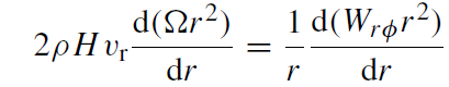
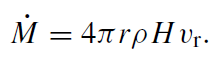
This model assumes the sub-mm and X-ray emission of Sgr A* arises from the circularization of the infalling gas at very small radii (Melia et al 2001). We construct a standard accretion disk with the assumption that turbulence produces a magnetic field that is predominantly azimuthal. We start with the solution to the Euler equation for inward viscous transport (Shakura and Sunyaev 1973) in a Keplerian disk,
 (1.1)
(1.1)
where vr is the (positive inward) radial velocity of the gas, H is the height of the disk,
 (1.2)
(1.2)
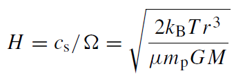
is the Keplerian rotational frequency, and Wrφ is the vertically integrated stress. We assume that vr << r Ω for all r . The disk height is found by balancing gravity with the vertical pressure gradient
 (1.3)
(1.3)
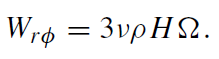
where cs is the isothermal sound speed. The stress is related to the kinematic shear viscosity ν by
 (1.4)
(1.4)
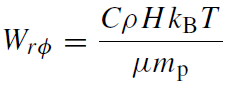
We assume the stress is dominated by the Maxwell stress so that if we assume the magnetic energy density scales with the thermal energy density, we have
 (1.5)
(1.5)
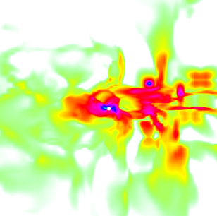
Figure 1.1. A plot of logarithmic density through the ˆ x–ˆz plane for a sample hydrodynamical simulation applicable to Sgr A*. The image is 16 RA  0.3 pc 106 rs on a side. The darkest color corresponds to a number density > 104 cm−3 and white corresponds to a number density < 102 cm−3. Sgr A* is modeled as a perfectly absorbing sphere with a radius of 0.1 RA. The 10 wind sources, one of which is visible to the upper right of Sgr A*, have been blowing for ∼2500 years.
where C is a constant scale factor. Numerical MHD simulations suggest C ∼ 0.01 (Brandenburg et al 1995). Note that with these definitions, C = 3α, where α is the standard Shakura-Sunyaev viscosity parameter. We also have the disk version of the mass continuity equation
 (1.6)
(1.6)
Together, this permits us to write the integral (1.1) as
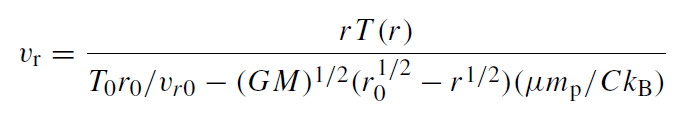 (1.7)
(1.7)
where the quantities with subscript 0 are evaluated at the outer edge of the disk (i.e. at radius r0). For (1.7) to represent a physical accretion solution, the denominator of (1.7) must not reach zero. Letting vr→∞at the inner edge of the disk (≡1 rs), we get T0 in terms of r0 and vr0:
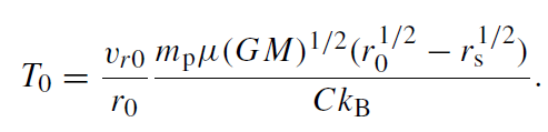 (1.8)
(1.8)
Turbulence with perturbing wavenumbers k Ω/vAz, where vAz is the Alfven velocity due to the vertical magnetic field, is unstable and generates a positive feedback loop between the kinetic energy density of the turbulence and the energy density of the turbulent magnetic field. This ‘dynamo’ turns off when the two energy densities are in rough equipartition. The net result is that the equilibrium magnetic energy density is a fraction βB ∼ 0.03 of the total thermal energy density. Many numerical simulations have verified this expectation (Hawley et al 1995). Also, the most unstable modes are not damped by Ohmic diffusion because the diffusion length for gas ∼10 rs from Sgr A* is extremely small (Melia et al 2001). Given the disparate stellar sources of the infalling gas, a dominant large-scale ordered magnetic field is unlikely. In such a case, the turbulent magnetic field will likely dominate the final magnetic energy density.
It remains to solve the total (magnetic, kinetic, and thermal) energy equation in order to derive the temperature profile. This requires solving the equation for thermal energy conservation as well as the magnetic evolution equation in the presence of Ohmic diffusion and viscous dissipation (Balbus and Hawley 1991):
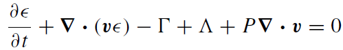 (1.9)
(1.9)
 (1.10)
where η is the resistivity of the fully ionized gas (Spitzer 1962). We assume azimuthal symmetry and incompressibility and neglect radiation pressure and buoyancy in order to find the steady-state solutions to (1.9) and (1.10). Since we are not using the relativistic Euler equation, the results will not be strictly valid near rs; more complicated corrections such as those due to light bending are also ignored.
The most difficult aspect of determining the accretion profiles is solving for the steady-state dissipative heating term, Γ, in terms of the current density and stress. This requires ignoring the divergence of the viscous and Ohmic fluxes and taking only the high-order terms. More details are given in Melia et al (2001) but the resulting differential equation for the temperature is
 (1.11)
where
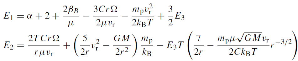
 (1.12)
Together with (1.6) and (1.7), equation (1.11) determines the accretion profile, provided some boundary conditions are given. An example of some profiles that may be applicable to Sgr A* are shown in figure 1.2. Note that while spherical accretion is always stable (Moncrief 1980), it has not been determined whether the disklike profiles given here produce a thermally or dynamically stable disk.
Calculation of the spectrum
We calculate the spectrum due to this Keplerian flow model in a fashion that parallels. At a frequency ν0, the predicted observed flux density produced by the Keplerian flow is given by
 (1.13)
where D = 8.5 kpc is the distance to the Galactic Center and the observed frequency at infinity is now
 (1.14)
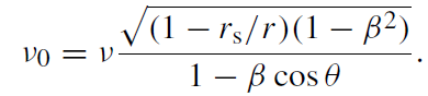
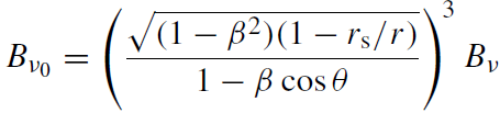
The term in (1.13) is due to the gravitational redshift. The frequency measured in the comoving frame is ν,
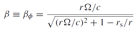 (1.15)
is the normalized azimuthal velocity seen by a stationary observer, and θ is the angle between β and the line of sight. Thus,
cos θ ≡ sin i cos φ (1.16)
where i is the inclination angle with respect to the line of sight of the rotation axis perpendicular to the Keplerian flow, and φ is the position angle of the emitting element. Figure 1.3 shows a cartoon of the accretion region. The area element is
 (1.17)

Figure 1.2. Example profiles for a Keplerian accretion with magnetic dynamo model for Sgr A*. Here ˙M = 1016 g s−1, vr0 = 5×10⁻⁴ vkep, C = 0.01, βB = 0.03, and r0 = 5 rs.
and the specific intensity
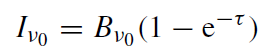 (1.18)
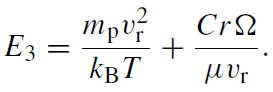
where
 (1.19)
and Bν is again the blackbody Planck function. The optical depth from the emitting element to the observer is approximately
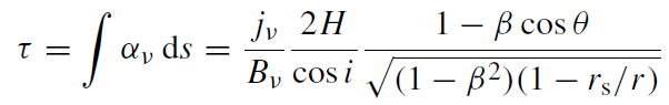 (1.20)
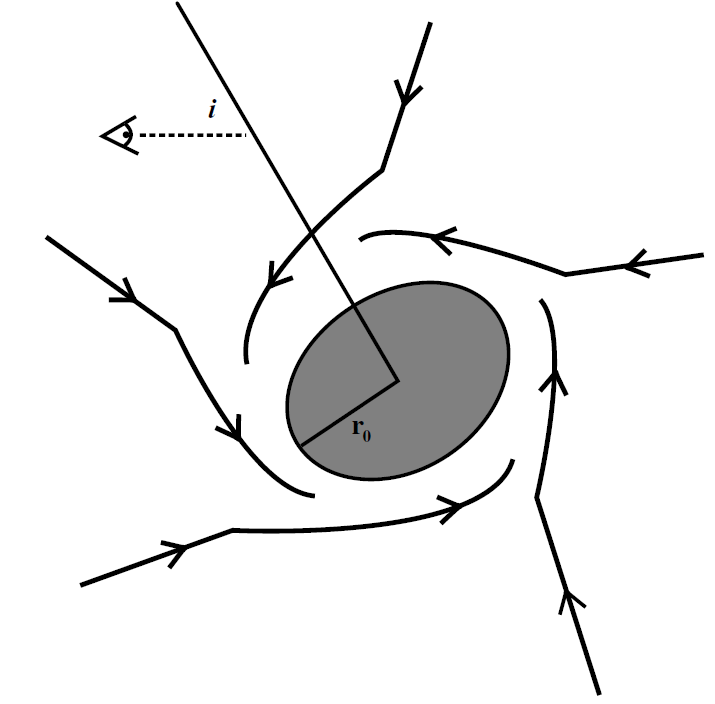
Figure 1.3. Schematic diagram showing streamlines of infalling gas for the Keplerian accretion model.
where jν is the emissivity in the comoving frame. Note that the transformations in these equations implicitly assume that βφ >> βr for all r . Given a prescription for the emissivity, this determines the spectrum.
There are some differences between the derivation here. The geometry of a disk instead of spherical inflow results in a different treatment of the optical depth. In a disk there is only local absorption as in (1.18) while in spherical flow a photon can be absorbed at large radii. Also, here we can no longer assume that cos φ = 0. Instead, it is necessary to explicitly integrate over φ.
An example of a spectrum, assuming an emissivity due to relativistic magnetic bremsstrahlung from thermal particles (Pacholczyk 1970), is given in figure 1.4. The input parameters are the same as for the profiles shown in figure 1.2. With some tuning, this model can reproduce the sub-mm ‘bump’ in the radio emission but has too steep a spectral index, resulting in very little
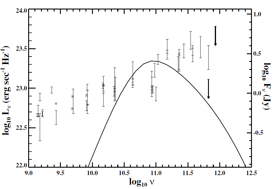
Figure 1.4. Example spectrum for a Keplerian accretion model for Sgr A* using the profiles shown in figure 1.2. Here we use a representative disk inclination of 60o.
low-frequency emission. As previously stated, this is expected for a thermal distribution of particles and implies that the low-frequency emission is distinct from the sub-mm. Perhaps the low-frequency radio emission originates in a small jet or further out in the semi-spherical accretion flow. The X-ray emission due to thermal bremsstrahlung from the model shown in figure 1.4 is considerably less than the detected X-ray flux. However, by including inverse Compton, which up scatters the sub-mm-wave photons, one can reproduce the observed flux and spectral index of the X-ray emission. The primary conclusion of this model is that in order to produce consistent radio emission without violating the IR or X-ray limits, one requires a mass accretion rate at ∼10 rs that is around three orders of magnitude less than that predicted from the simple Bondi–Hoyle estimate. Given the good constraints on the large-scale winds, this implies a strongly radially dependent mass accretion rate. Also, the lower mass accretion rate results in a higher final radiative efficiency of 7%, about that expected for accretion disk scenarios.


|
|
|
|
تفوقت في الاختبار على الجميع.. فاكهة "خارقة" في عالم التغذية
|
|
|
|
|
|
|
أمين عام أوبك: النفط الخام والغاز الطبيعي "هبة من الله"
|
|
|
|
|
|
|
قسم شؤون المعارف ينظم دورة عن آليات عمل الفهارس الفنية للموسوعات والكتب لملاكاته
|
|
|