
آخر المواضيع المضافة

 الفيزياء الكلاسيكية
الكهربائية والمغناطيسية
علم البصريات
الفيزياء الحديثة
النظرية النسبية
الفيزياء النووية
فيزياء الحالة الصلبة
الليزر
علم الفلك
المجموعة الشمسية
الطاقة البديلة
الفيزياء والعلوم الأخرى
مواضيع عامة في الفيزياء
الفيزياء الكلاسيكية
الكهربائية والمغناطيسية
علم البصريات
الفيزياء الحديثة
النظرية النسبية
الفيزياء النووية
فيزياء الحالة الصلبة
الليزر
علم الفلك
المجموعة الشمسية
الطاقة البديلة
الفيزياء والعلوم الأخرى
مواضيع عامة في الفيزياء| Ludwig Boltzmann |


|
|
Read More
Date: 18-10-2015
Date: 9-11-2015
Date: 9-12-2015
|
Ludwig Boltzmann
The Story of e
Functions containing e are ubiquitous in the equations of physics. Prototypes are the “exponential functions” ex and e-x. Both are plotted in figure 1.1, showing that ex increases rapidly as x increases (“exponential increase” is a popular phrase), and e-x decreases rapidly. The constant e may seem mystifying. Where does it come from? Why is it important?
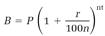
Mathematicians include e in their pantheon of fundamental numbers, along with 0, 1, π, and i. The use of e as a base for natural logarithms dates back to the seventeenth century. Eli Maor speculates that the definition of e evolved somewhat earlier from the formulas used for millennia by moneylenders. One of these calculates the balance B from the principal P at the interest rate r for a period of t years compounded n times a year,
 (1)
(1)
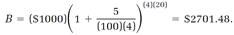
For example, if we invest P = $1000 at the interest rate r = 5% with interest compounded quarterly (n = 4), our balance after t = 20 years is
Equation (1) has some surprising features that could well have been noticed by an early-seventeenth-century mathematician. Suppose we simplify the formula by considering a principal of P = $1, a period of t = 1 year, and an interest rate of r = 100% (here we part with reality), so the right side of the formula is
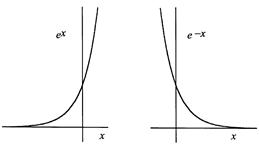
Figure 1.1. Typical exponential functions: the increasing ex and the decreasing e-x.
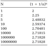
simply (1+1/n)n. Our seventeenth-century mathematician might have amused himself by laboriously calculating according to this recipe with n given larger and larger values (easily done with a calculator by using the yx key to calculate the powers). Table 1.1 lists some results. The trend is clear: the effect of increasing n becomes more minuscule as n gets larger, and as (1-1/n)n approaches a definite value, which is 2.71828 if six digits are sufficient. (For more accuracy, make n larger.) The “limit” approached when n is given an infinite value is the mathematical definition of the number e. Mathematicians write the definition
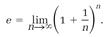 . (2)
. (2)
Physicists, chemists, engineers, and economists find many uses for exponential
functions of the forms ex and e-x. Here are a few of them:
1. When a radioactive material decays, its mass decreases exponentially according to

in which m is the mass at time t, m0 is the initial mass at time t = 0, and a is a constant that depends on the rate of decay of the radioactive material. The exponential factor e-at is rapidly decreasing (a is large) for short-lived radioactive materials, and slowly decreasing (a is small) for long-lived materials.
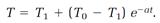
2. A hot object initially at the temperature T0 in an environment kept at the lower, constant temperature T1 cools at a rate given by
3. When a light beam passes through a material medium, its intensity decreases exponentially according to

Table 1.1
in which I is the intensity of the beam after passing through the thickness x of the medium, I0 is the intensity of the incident beam, and a is a constant depending on the transparency of the medium.
4. Explosions usually take place at exponentially increasing rates expressed by a factor of the form eat, with a a positive constant depending on the physical and chemical mechanism of the explosion.
5. If a bank could be persuaded to compound interest not annually, semiannually, or quarterly, but instantaneously, one's balance B would increase exponentially according to

where P is the principle, r is the annual interest rate, and t is the time in years.
Brickbats and Molecules
The story of statistical mechanics has an unlikely beginning with a topic that has fascinated scientists since Galileo's time: Saturn's rings. In the eighteenth century, Pierre-Simon Laplace developed a mechanical theory of the rings and surmised that they owed their stability to irregularities in mass distribution. The biennial Adams mathematical prize at Cambridge had as its subject in 1855 “The Motions of Saturn's Rings.” The prize examiners asked contestants to evaluate Laplace's work and to determine the dynamical stability of the rings modeled as solid, fluid, or “masses of matter not mutually coherent.” Maxwell entered the competition, and while he was at Aberdeen, devoted much of his time to it.
He first disposed of the solid and fluid models, showing that they were not stable or not flat as observed. He then turned to the remaining model, picturing it as a “flight of brickbats” in orbit around the planet. In a letter to Thomson, he said he saw it as “a great stratum of rubbish jostling and jumbling around Saturn without hope of rest or agreement in itself, till it falls piecemeal and grinds a fiery ring round Saturn's equator, leaving a wide tract of lava and dust and blocks on each side and the western side of every hill buttered with hot rocks. . . . As for the men of Saturn I should recommend them to go by tunnel when they cross the ‘line.’ ” In this chaos of “rubbish jostling and jumbling” Maxwell found a solution to the problem that earned the prize.
This success with Saturn's chaos of orbiting and colliding rocks inspired Max well to think about the chaos of speeding and colliding molecules in gases. At first, this problem seemed too complex for theoretical analysis. But in 1859, just as he was completing his paper on the rings, he read two papers by Clausius that gave him hope. Clausius had brought order to the molecular chaos by making his calculations with an average dynamical property, specifically the average value of v2, the square of the molecular velocity. Clausius wrote this average quantity  and used it in the equation
 (3)
(3)
to calculate the pressure P produced by N molecules of mass m randomly bombarding the walls of a container whose volume is V.
In Clausius's treatment, the molecules move at high speeds but follow extremely tortuous paths because of incessant collisions with other molecules. With all the diversions, it takes the molecules of a gas a long time to travel even a few meters. As Maxwell put it: “If you go 17 miles per minute and take a totally new course [after each collision] 1,700,000,000 times in a second where will you be in an hour?”
Maxwell's first paper on the dynamics of molecules in gases in 1860 took a major step beyond Clausius's method. Maxwell showed what Clausius recognized but did not include in his theory: that the molecules in a gas at a certain temperature have many different speeds covering a broad range above and below the average value. His reasoning was severely abstract and puzzling to his contemporaries, who were looking for more-mechanical details. As Maxwell said later in a different context, he did not make “personal enquiries [concerning the molecules], which would only get me in trouble.”
Maxwell asked his readers to consider the number of molecules dN with velocity components that lie in the specific narrow ranges between vx and vx + dvx, vy and vy + dvy, vz and vz + dvz. That count depends on N, the total number of molecules; on dvx, dvy, and dvz; and on three functions of vx, vy, and vz, call them f (vx), f (vy), and f (vz), expressing which velocity components are important and which unimportant. If, for example, vx = 10 meters per second is unlikely while vx = 500 meters per second is likely, then f (vx) for the second value of vx is larger than it is for the first value. Maxwell's equation for dN was
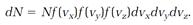 (4)
(4)
Maxwell argued that on the average in an ideal gas the three directions x, y, and z, used to construct the velocity components vx, vy, and vz, should all have the same weight; there is no reason to prefer one direction over the others. Thus the three functions f (vx), f (vy), and f (vz) should all have the same mathematical form. From this conclusion, and the further condition that the total number of molecules N is finite, he derived
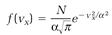 (5)
(5)
with α a parameter depending on the temperature and the mass of the molecules. This is one version of Maxwell's “distribution function.”
A more useful result, expressing the distribution of speeds v, regardless of direction, follows from this one,
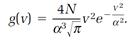 (6)
(6)
The function, g(v), another distribution function, assesses the relative importance of the speed v. Its physical meaning is conveyed in figure 1.2, where g(v) is plotted for speeds of carbon dioxide molecules ranging from 0 to 1,400 meters per second; the temperature is assumed to be 500 on the absolute scale (227oC). We can see from the plot that very high and very low speeds are unlikely, and that the most probable speed at the maximum point on the curve is about 430 meters per second (= 16 miles per minute).
Maxwell needed only one page in his 1860 paper to derive the fundamental equations (5) and (6) as solutions to the proposition “To find the average number of particles [molecules] whose velocities lie between given limits, after a great number of collisions among a great number of equal particles.” The language calculation of an “average” for a “great number” of molecules and collisions prescribes a purely statistical description, and that is what Maxwell supplied in his distribution functions.
Thus, without “personal enquiries” into the individual histories of molecules, Maxwell defined their statistical behavior instead, and this, he demonstrated in his 1860 paper, had many uses. Statistically speaking, he could calculate for a gas its viscosity, ability to conduct heat, molecular collision rate, and rate of diffusion. This was the beginning “of a new epoch in physics,” C. W. F. Everitt writes. “Statistical methods had long been used for analyzing observations, both in physics and in the social sciences, but Maxwell’s ideas of describing actual physical processes by a statistical function [e.g., g(v) in equation (6)] was an extraordinary novelty.”
Maxwell's theory predicted, surprisingly, that the viscosity parameter for gases
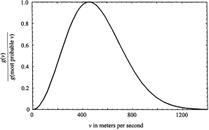
Figure 1.2. Maxwell’s distribution function g(v). The plot is “normalized” by dividing each value of g(v) by the value obtained with v given its most probable value.
should be independent of the pressure of the gas. “Such a consequence of a mathematical theory is very startling,” Maxwell wrote, “and the only experiment I have met with on the subject does not seem to confirm it.” His convictions were with the theory, however, and several years later, ably assisted by his wife Katherine, Maxell demonstrated the pressure independence experimentally. Once more, the scientific community was impressed by Maxwellian wizardry.
But the theory could not explain some equally puzzling data on specific heats. A specific heat measures the heat input required to raise the temperature of one unit, say, one kilogram, of a material one degree. Measurements of specific heats can be done for constant-pressure and constant-volume conditions, with the former always larger than the latter.
Maxwell, like many of his contemporaries, believed that heat resides in molecular motion, and therefore that a specific heat reflects the number of modes of molecular motion activated when a material is heated. Maxwell's theory supported a principle called the “equipartition theorem,” which asserts that the thermal energy of a material is equally divided among all the modes of motion belonging to the molecules. Given the number of modes per molecule, the theory could calculate the constant-pressure and constant-volume specific heats and the ratio between the two. If the molecules were spherical, they could move in straight lines and also rotate. Assuming three (x, y, and z) components for both rotation and straight-line motion, the tally for the equipartition theorem was six, and the prediction for the specific-heat ratio was 1.333. The observed average for several gases was 1.408.
Maxwell never resolved this problem, and it bothered him throughout the 1870s. In the end, his advice was to regard the problem as “thoroughly conscious ignorance,” and expect that it would be a “prelude to [a] real advance in knowledge.” It was indeed. Specific-heat theory remained a puzzle for another twenty years, until quantum theory finally explained the mysterious failings of the equipartition theorem.
Entropy and Disorder
We come now to Boltzmann's role in the development of statistical mechanics, supporting and greatly extending the work already done by Clausius and Maxwell. Boltzmann's first major contribution, in the late 1860s, was to broaden Maxwell's concept of a molecular distribution function. He established that the factor for determining the probability that a system of molecules has a certain total (kinetic + potential) energy E is proportional to e-hE, with h a parameter that depends only on temperature. This “Boltzmann factor” has become a fixture in all kinds of calculations that depend on molecular distributions, not only for physicists but also for chemists, biologists, geologists, and meteorologists.
Boltzmann assumed that his statistical factor operates in a vast “phase space” spanning all the coordinates and all the velocity components in the system. Each point in the phase space represents a possible state of the system in terms of the locations of the molecules and their velocities. As the system evolves, it follows a path from one of these points to another.
Boltzmann constructed his statistical theory by imagining a small element, call it d⍵, centered on a point in phase space, and then assuming that the probability dP for the system to be in a state represented by points within an element is proportional to the statistical factor e-hE multiplied by the element d⍵:

or
 (7)
(7)
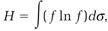
where A is a proportionality constant. Probabilities are always defined so that when they are added for all possible events they total one. Doing the addition of the above dPs with an integration, we have

so integration of both sides of equation (7),
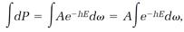
leads to
and this evaluates the proportionality constant A,
 (8)
(8)
Substituting in equation (7), we have
 (9)
(9)
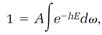
This is an abstract description, but it is also useful. If we can express any physical quantity, say the entropy S, as a function of the molecular coordinates and velocities, then we can calculate the average entropy  statistically by simply multiplying each possible value of S by its corresponding probability dP, and adding by means of an integration,
 (10)
(10)
So far, Boltzmann's statistical treatment was limited in that it concerned reversible processes only. In a lengthy and difficult paper published in 1872, Boltzmann went further by building a molecular theory of irreversible processes. He began by introducing a molecular velocity distribution function f that resembled Maxwell's function of the same name and symbol, but that was different in the important respect that Boltzmann's version of f could evolve: it could change with time.
Boltzmann firmly believed that chaotic collisions among molecules are responsible for irreversible changes in gaseous systems. Taking advantage of a mathematical technique developed earlier by Maxwell, he derived a complicated equation that expresses the rate of change in f resulting from molecular collisions. The equation, now known as the Boltzmann equation, justifies two great propositions. First, it shows that when f has the Maxwellian form seen in equation (5) its rate of change equals zero. In this sense, Maxwell's function expresses a static or equilibrium distribution.
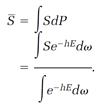
Second, Boltzmann's equation justifies the conclusion that Maxwell's distribution function is the only one allowed at equilibrium. To make this point, he introduced a time-dependent function, which he later labeled H,
 (11)
(11)
in which dσ = dvxdvydvz. The H-function, teamed with the Boltzmann equation, leads to Boltzmann's “H-theorem,” according to which H can never evolve in an increasing direction: the rate of change in H, that is, the derivative dH/dt, is either negative (H decreasing) or zero (at equilibrium),
 (12)
(12)
Thus the H-function follows the irreversible evolution of a gaseous system, always decreasing until the system stops changing at equilibrium, and there Boltzmann could prove that f necessarily has the Maxwellian form.
As Boltzmann's H-function goes, so goes the entropy of an isolated system according to the second law, except that H always decreases, while the entropy S always increases. We allow for that difference with a minus sign attached to H and conclude that
 (13)
(13)
In this way, Boltzmann's elaborate argument provided a molecular analogue of both the entropy concept and the second law.
There was, however, an apparent problem. Boltzmann's argument seemed to be entirely mechanical in nature, and in the end to be strictly reliant on the Newtonian equations of mechanics or their equivalent. One of Boltzmann's Vienna colleagues, Joseph Loschmidt, pointed out (in a friendly criticism) that the equations of mechanics have the peculiarity that they do not change when time is reversed: replace the time variable t with –t, and the equations are unchanged. In Loschmidt's view, this meant that physical processes could go backward or forward with equal probability in any mechanical system, including Boltzmann's assemblage of colliding molecules. One could, for example, allow the molecules of a perfume to escape from a bottle into a room, and then expect to see all of the molecules turn around and spontaneously crowd back into the bottle. This was completely contrary to experience and the second law. Loschmidt concluded that Boltzmann's molecular interpretation of the second law, with its mechanical foundations, was in doubt.
Boltzmann replied in 1877 that his argument was not based entirely on mechanics: of equal importance were the laws of probability. The perfume molecules could return to the bottle, but only against stupendously unfavorable odds. He made this point with an argument that turned out to be cleverer than he ever had an opportunity to realize. He proposed that the probability for a certain physical state of a system is proportional to a count of “the number of ways the inside [of the system] can be arranged so that from the outside it looks the same,” as Richard Feynman put it. To illustrate what this means, imagine two vessels like those guarded by Maxwell's demon. The entire system, including both vessels, contains two kinds of gaseous molecules, A and B. We obtain Boltzmann's count by systematically enumerating the number of possible arrangements of molecules between the vessels, within the restrictions that the total number of molecules does not change, and the numbers of molecules in the two vessels are always the same.
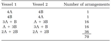
The pattern of the calculation is easy to see by doing it first for a ridiculously small number of molecules, and then extrapolating with the rules of “combinatorial” mathematics to systems of realistic size. Suppose, then, we have just eight non-interacting molecules, four As and four Bs, with four molecules (either A or B) in each vessel. One possibility is to have all the As in vessel 1 and all the Bs in vessel 2. This allocation can also be reversed: four As in vessel 2 and four Bs in vessel 1. Two more possibilities are to have three As and one B in vessel 1, together with one A and three Bs in vessel 2, and then the reverse of this allocation. The fifth, and last, allocation is two As and two Bs in both vessels; reversing this allocation produces nothing new. These five allocations are listed in Table 1.2 in the first two columns.
Boltzmann asks us to calculate the number of molecular arrangements allowed by each of these allocations. If we ignore rearrangements within the vessels, the first two allocations are each counted as one arrangement. The third allocation has more arrangements because the single B molecule in vessel 1 can be any one of the four Bs, and the single A molecule in vessel 2 can be any of the four As. The total number of arrangements for this allocation is 4 × 4 = 16. Arrangements for the fourth allocation are counted similarly. The tally for the fifth allocation (omitting the details) is 36. Thus for our small system the total “number of ways the inside can be arranged so that from the outside it looks the same,” a quantity we will call W, is
W = 1 + 1 + 16 + 16 + 36 = 70.
Table 1.2
This result can be obtained more abstractly, but with much less trouble, by taking advantage of a formula from combinatorial mathematics,
 (14)
(14)
where N = NA + NB and the “factorial” notation ! denotes a sequence of products such as 4! = 1•2•3•4. For the example, NA = 4, NB = 4, N = NA + NB = 8, and
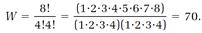
In Boltzmann's statistical picture, our very small system wanders from one of the seventy arrangements to another, with each arrangement equally probable. About half the time, the system chooses the fifth allocation, in which the As and Bs are completely mixed, but there are two chances in seventy that the system will completely unmix by choosing the first or the second allocation. An astonishing thing happens if we increase the size of our system. Suppose we double the size, so NA = 8, NB = 8, N = NA + NB = 16, and
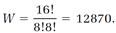
There are now many more arrangements possible. We can say that the system has become much more “disordered.” As is now customary, we will use the term “disorder” for Boltzmann's W.
The beauty of the combinatorial formula (14) is that it applies to a system of any size, from microscopic to macroscopic. We can make the stupendous leap from an N absurdly small to an N realistically large and still trust the simple combinatorial calculation. Suppose a molar amount of a gas is involved, so N = 6 × 10²³, NA = 3 × 10²³, NB = 3 × 10²³, and
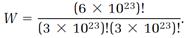
The factorials are now enormous numbers, and impossible to calculate directly. But an extraordinarily useful approximation invented by James Stirling in the eighteenth century comes to the rescue: if N is very large (as it certainly is in our application) then
ln N! = Nln N - N.
Applying this shortcut to the above calculation of the disorder W, we arrive at
lnW = 4 × 10²³
or
W = e4 × 1023.
This is a fantastically large number; its exponent is 4 × 10²³. We cannot even do it justice by calling it astronomical. This is the disorder that is, the total number of arrangements in a system consisting of 1⁄2 mole of one gas thoroughly mixed with 1⁄2 mole of another gas. In one arrangement out of this incomprehensibly large number, the gases are completely unmixed. In other words, we have one chance in e4 × 1023 to observe the unmixing. There is no point in expecting that to happen. Now it is clear why, according to Boltzmann, the perfume molecules do not voluntarily unmix from the air in the room and go back into the bottle.
Boltzmann found a way to apply his statistical counting method to the distribution of energy to gas molecules. Here he was faced with a special problem: he could enumerate the molecules themselves easily enough, but there seemed to be no natural way to count the “molecules” of energy. His solution was to assume as a handy fiction that energy was parceled out in discrete bundles, later called energy “quanta,” all carrying the same very small amount of energy. Then, again following the combinatorial route, he analyzed the statistics of a certain number of molecules competing for a certain number of energy quanta. He found that a particular energy distribution, the one dictated by his exponential factor e-hE, overwhelmingly dominates all the others. This is, by an immense margin, the most probable energy distribution, although others are possible.
Boltzmann also made the profound discovery that when he allowed his energy quanta to diminish to zero size, the logarithm of his disorder count W was proportional to his H-function inverted with a minus sign, that is,
 (15)
(15)
Then, in view of the connection between the H-function and entropy (the proportionality (13)), he arrived at a simple connection between entropy and disorder,
 (16)
(16)
Boltzmann's theoretical argument may seem abstract and difficult to follow, but his major conclusion, the entropy-disorder connection, is easy to comprehend, at least in a qualitative sense. Order and disorder are familiar parts of our lives, and consequently so is entropy. Water molecules in steam are more disordered than those in liquid water (at the same temperature), and water molecules in the liquid are in turn more disordered than those in ice. As a result, steam has a larger entropy than liquid water, which has a larger entropy than ice (if all are at the same temperature). When gasoline burns, the order and low entropy of large molecules such as octane are converted to the disorder and higher entropy of smaller molecules, such as carbon dioxide and water, at high temperatures. A pack of cards has order and low entropy if the cards are sorted, and disorder and higher entropy if they are shuffled. Our homes, our desks, even our thoughts have order or disorder. And entropy is there too, rising with disorder, and falling with order.
Entropy and Probability
We can surmise that Gibbs developed his ideas on statistical mechanics more or less in parallel with Boltzmann, although in his deliberate way Gibbs had little to say about the subject until he published his masterpiece, Elementary Principles in Statistical Mechanics, in 1901. That he was thinking about the statistical interpretation of entropy much earlier is clear from his incidental remark that “an uncompensated decrease of entropy seems to be reduced to improbability.” As mentioned, Gibbs wrote this in 1875 in connection with a discussion of the mixing and unmixing of gases. Gibbs's speculation may have helped put Boltzmann on the road to his statistical view of entropy; at any rate, Boltzmann included the Gibbs quotation as an epigraph to part 2 of his Lectures on Gas Theory, written in the late 1890s.
Gibbs's Elementary Principles brought unity to the “gas theory” that had been developed by Boltzmann, Maxwell, and Clausius, supplied it with the more elegant name “statistical mechanics,” and gave it a mathematical style that is preferred by today's theorists. His starting point was the “ensemble” concept, which Maxwell had touched on in 1879 in one of his last papers. The general idea is that averaging among the many states of a molecular system can be done conveniently by imagining a large collection an ensemble of replicas of the system, with the replicas all exactly the same except for some key physical properties. Gibbs proposed ensembles of several different kinds; the one I will emphasize he called “canonical.” All of the replicas in a canonical ensemble have the same volume and temperature and contain the same number of molecules, but may have different energies.
Averaging over a canonical ensemble is similar to Boltzmann's averaging procedure. Gibbs introduced a probability P for finding a replica in a certain state, and then, as in Boltzmann's equation (7), he calculated the probability dP that the system is located in an element of phase space,
dP = Pd⍵. (17)
These probabilities must total one when they are added by integration,
 (18)
(18)
Gibbs, like Boltzmann, was motivated by a desire to compose a statistical molecular analogy with thermodynamics. Most importantly, he sought a statistical entropy analogue. He found that the simplest way to get what he wanted from a canonical ensemble was to focus on the logarithm of the probability, and he introduced
S = = k lnP (19)
for the entropy of one of the replicas belonging to a canonical ensemble. The constant k (Gibbs wrote it 1/K) is a very small number with the magnitude 1.3807 ×10⁻²³ if the energy unit named after Joule is used. It is now known as “Boltzmann's constant” (although Boltzmann did not use it, and Max Planck was the first to recognize its importance).
In Gibbs's scheme, as in Boltzmann's, the probability P is a mathematical tool for averaging. To calculate an average energy  we simply multiply each energy E found in a replica by the corresponding probability dP = Pd⍵ and add by integrating
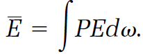 (20)
(20)
The corresponding entropy calculation averages the entropies for the replicas given by equation (19),
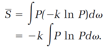 (21)
(21)
The constant k is pervasive in statistical mechanics. It not only serves in Gibbs's fundamental entropy equations, but it is also the constant that makes Boltzmann's entropy proportionality (16) into one of the most famous equations in physics,
S = k lnW. (22)
The equation is carved on Boltzmann's grave in Vienna's Central Cemetery (in spite of the anachronistic k).
We now have two statistical entropy analogues, Gibbs's and Boltzmann's, expressed in equations (21) and (22). The two equations are obviously not mathematically the same. Yet they apparently calculate the same thing, entropy. One difference is that Gibbs used probabilities P, quantities that are always less than one, while Boltzmann based his calculation on the disorder W, which is larger than one (usually much larger). It can be proved (in more space than we have here) that the two equations are equivalent if the system of interest has a single energy.
Gibbs proved that a system represented by his canonical ensemble does have a fixed energy to an extremely good approximation. He calculated the extent to which the energy fluctuates from its average value. For the average of the square of this energy fluctuation he found kT2Cv, where k is again Boltzmann's constant, T is the absolute temperature, and Cv is the heat capacity (the energy required to increase one mole of the material in the system by one degree) measured at constant volume. Neither T nor Cv is very large, but k is very small, so the energy fluctuation is also very small. A similar calculation of the entropy fluctuation gave kCv, also very small.
Thus the statistical analysis, either Gibbs's or Boltzmann's, arrives at an energy and entropy that are, in effect, constant. They are, as Gibbs put it, “rational foundations” for the energy and entropy concepts of the first and second laws of thermodynamics.
Note one more important use of the ever-present Boltzmann constant k. Gibbs proved that the h factor appearing in Boltzmann's statistical factor e-hE is related to the absolute temperature T by h = 1/kT, so the Boltzmann factor, including the temperature, is e-E/kT.


|
|
|
|
إجراء أول اختبار لدواء "ثوري" يتصدى لعدة أنواع من السرطان
|
|
|
|
|
|
|
دراسة تكشف "سببا غريبا" يعيق نمو الطيور
|
|
|
|
|
|
لأعضاء مدوّنة الكفيل السيد الصافي يؤكّد على تفعيل القصة والرواية المجسّدة للمبادئ الإسلامية والموجدة لحلول المشاكل المجتمعية
|
|
|
|
قسم الشؤون الفكرية يناقش سبل تعزيز التعاون المشترك مع المؤسّسات الأكاديمية في نيجيريا
|
|
|
|
ضمن برنامج عُرفاء المنصّة قسم التطوير يقيم ورشة في (فنّ الٕالقاء) لمنتسبي العتبة العباسية
|
|
|
|
وفد نيجيري يُشيد بمشروع المجمع العلمي لحفظ القرآن الكريم
|