Wave Equation-1-Dimensional
The one-dimensional wave equation is given by
 |
(1)
|
In order to specify a wave, the equation is subject to boundary conditions
and initial conditions
The one-dimensional wave equation can be solved exactly by d'Alembert's solution, using a Fourier transform method, or via separation of variables.
d'Alembert devised his solution in 1746, and Euler subsequently expanded the method in 1748. Let
By the chain rule,
The wave equation then becomes
 |
(10)
|
Any solution of this equation is of the form
 |
(11)
|
where  and
and  are any functions. They represent two waveforms traveling in opposite directions,
  in the negative
  direction and
  in the positive
  direction.
The one-dimensional wave equation can also be solved by applying a Fourier transform to each side,
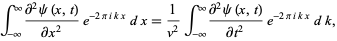 |
(12)
|
which is given, with the help of the Fourier transform derivative identity, by
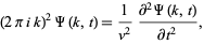 |
(13)
|
where
This has solution
 |
(16)
|
Taking the inverse Fourier transform gives
where
This solution is still subject to all other initial and boundary conditions.
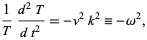
The one-dimensional wave equation can be solved by separation of variables using a trial solution
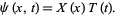 |
(23)
|
This gives
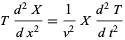 |
(24)
|
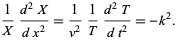 |
(25)
|
So the solution for  is
is
 |
(26)
|
Rewriting (25) gives
 |
(27)
|
so the solution for  is
is
 |
(28)
|
where  . Applying the boundary conditions
 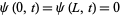 to (◇) gives
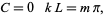 |
(29)
|
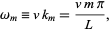
where  is an integer. Plugging (◇), (◇) and (29) back in for
  in (◇) gives, for a particular value of
  ,
,
The initial condition  then gives
  , so (31) becomes
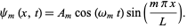 |
(32)
|
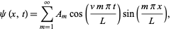
The general solution is a sum over all possible values of  , so
, so
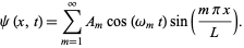 |
(33)
|
Using orthogonality of sines again,
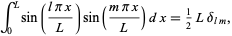 |
(34)
|
where  is the Kronecker delta defined by
![delta_(mn)=<span style=]() {1 m=n; 0 m!=n, " src="http://mathworld.wolfram.com/images/equations/WaveEquation1-Dimensional/NumberedEquation17.gif" style="height:41px; width:109px" /> {1 m=n; 0 m!=n, " src="http://mathworld.wolfram.com/images/equations/WaveEquation1-Dimensional/NumberedEquation17.gif" style="height:41px; width:109px" /> |
(35)
|
gives
so we have
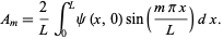 |
(39)
|
The computation of  s for specific initial distortions is derived in the Fourier sine series section. We already have found that
  , so the equation of motion for the string (◇), with
 |
(40)
|
is
 |
(41)
|
where the  coefficients are given by (◇).
A damped one-dimensional wave
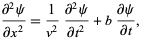 |
(42)
|
given boundary conditions
initial conditions
and the additional constraint
 |
(47)
|
can also be solved as a Fourier series.
![psi(x,t)=sum_(n=1)^inftysin((npix)/L)e^(-v^2bt/2)[a_nsin(mu_nt)+b_ncos(mu_nt)],](http://mathworld.wolfram.com/images/equations/WaveEquation1-Dimensional/NumberedEquation23.gif) |
(48)
|
where
REFERENCES:
Abramowitz, M. and Stegun, I. A. (Eds.). "Wave Equation in Prolate and Oblate Spheroidal Coordinates." §21.5 in Handbook of Mathematical Functions with Formulas, Graphs, and Mathematical Tables, 9th printing. New York: Dover, pp. 752-753, 1972.
Morse, P. M. and Feshbach, H. Methods of Theoretical Physics, Part I. New York: McGraw-Hill, pp. 124-125 and 271, 1953.
Zwillinger, D. (Ed.). CRC Standard Mathematical Tables and Formulae. Boca Raton, FL: CRC Press, p. 417, 1995.
Zwillinger, D. Handbook of Differential Equations, 3rd ed. Boston, MA: Academic Press, p. 130, 1997.


