We saw that the ten Einstein equations decompose into two sets of four and six equations respectively, four constraints which the initial data have to satisfy, and six equations driving the evolution. As a consequence, there will be four dynamically undetermined components among the ten components of the gravitational field g_μν. The task is to parametrize the g_μν in such a way that four dynamically undetermined functions can be cleanly separated from the other six. One way to achieve this is via the splitting of spacetime into space and time. The four dynamically undetermined quantities will be the famous lapse (one function α) and shift (three functions βⁱ ). The dynamically determined quantity is the Riemannian metric h_{i j} on the spatial three manifolds of constant time. These together parametrize g_μν as follows:

 (1.1)

The physical interpretation of α and βⁱ is: think of spacetime as the history of space. Each ‘moment’ of time, x⁰ = t, corresponds to an entire three-dimensional slice Σ_t . Obviously there is plenty of freedom in how to ‘waft’ space through spacetime. This freedom corresponds precisely to the freedom to choose the 1+3 functions α and βⁱ . For one thing, you may freely specify how far for each parameter step dt you push space in a perpendicular direction forward in time. This is controlled by α, which is just the ratio ds/dt of the proper perpendicular distance between the hypersurfaces Σ_t and Σ_t+dt . This speed may be chosen in a space and time-dependent fashion, which makes α a function on spacetime. Second, let a point be given with coordinates xⁱ on Σ_t . Going from xi in a perpendicular direction you meet Σ_t+dt in a point with coordinates xⁱ + dxⁱ , where dxⁱ can be chosen at will. This freedom of moving the coordinate system around while evolving is captured by βⁱ ; one writes dxⁱ = βⁱdt. Clearly this moving around of the spatial coordinates can also be made in a space- and time dependent fashion, so that the βⁱ are functions of spacetime, too.

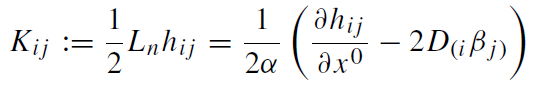
Let n^μ be the vector field in a spacetime which is normal to the spatial sections of constant time. It is given by n = 1/α (∂/∂x⁰ − βⁱ∂/∂xⁱ ), as one may readily verify by using (1.1) (you have to check that n is normalized and satisfies       g(n, ∂/∂xⁱ ) = 0). We define the extrinsic curvature, K^{i j} , to be one half the Lie derivative of the spatial metric in the direction of the normal:

 (1.2)

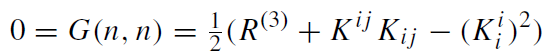
where D is the spatial covariant derivative with respect to the metric h_{i j}. As usual, a round bracket around indices denotes their symmetrization. Note that, by definition, K_{i j} is symmetric. Finally we denote the Ricci scalar of h_{i j} by R(3). We can now write down the four constraints of the vacuum Einstein equations in terms of these variables:

 (1.3)

 (1.4)

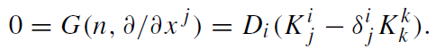
Equations (1.3) and (1.4) are referred to as the Hamiltonian constraint and momentum constraint, respectively. The six evolution equations of second order in the time derivative can now be written as 12 equations of first order. Six of them are just (1.2), read as the equation that relates the time derivative ∂h_{i j} /∂x⁰ to the ‘canonical data’ (h_{i j} , K_{i j} ). The other six equations, whose explicit form needs not concern us here, express the time derivative of K_{i j} in terms of the canonical data. Both sets of evolution equations contain, on their right-hand sides, the lapse and shift functions, whose evolution is not determined but must be specified by hand. This specification is a choice of gauge, without which one cannot determine the evolution of the physical variables (h_{i j} , K_{i j} ).

The initial data problem takes now the following form:

(1) Choose a topological three manifold Σ.

(2) Find on Σ a Riemannian metric h_{i j} and a symmetric tensor field K_{i j} which satisfy the constraints (1.3) and (1.4).

(3) Choose a lapse function α and a shift vector field βⁱ , both as functions of space and time, possibly according to some convenient prescription (e.g. singularity avoiding gauges, like maximal slicing).

(4) Evolve initial data with these choices of α and βⁱ according to the 12 equations of first order. By consistency of Einstein’s equations, the constraints will be preserved during this evolution, independent of the choices for α and βⁱ .

The backbone of this setup is a mathematical theorem, which states that for any set of initial data, taken from a suitable function space, there is, up to a diffeomorphism, a unique maximal Einstein spacetime developing.

اخر الاخبار

اخبار العتبة العباسية المقدسة

قسم الإعلام يشارك في الاجتماع التحضيري لمناقشة الخطة الإعلامية لزيارة عاشوراء

بحضور متوليها الشرعي.. العتبة العباسية المقدسة تواصل إقامة المجالس الحسينية لإحياء شهر المحرم

قسم الشؤون الفكرية يطلق برنامجه التبليغي في أكثر من 20 دولة إفريقية

شعبتا الخطابة النسوية والتوجيه الديني تواصلان إقامة المجالس الحسينية في مرقد أبي الفضل العباس (عليه السلام)

المزيد

الآخبار الصحية

دراسة تكشف علاقة خطيرة بين عمر الأم وصحة مولودها

دراسة تحذر.. اضطراب نوم بسيط قد يسبب الموت المبكر ؟

الاستحمام بالماء الساخن.. راحة مؤقتة وأضرار دائمة للبشرة

ماذا يحدث للجسم عند تخطي وجبة الإفطار؟

المزيد

الآخبار التكنلوجية

كيف تساعد الصيانة الوقائية في الحفاظ على كفاءة التكييف في سيارتك ؟

في ظاهرة غريبة حيرت العلماء.. كوكبنا قد يسجل أقصر يوم في التاريخ هذا الصيف!

السد الصيني العملاق يعيق دوران الأرض ويغيّر شكلها ؟

السعودية تطلق 10 تجارب علمية إلى محطة الفضاء الدولية

المزيد

مواضيع ذات صلة

الأسرار المتبقية للثقوب السوداء ( نهاية الزمكان أم بوابة لكون آخر؟)

الثقوب الدودية

الثقوب البيضاء

الثقوب السوداء العملاقة

الثقوب السوداء

الثقوب السوداء

الطبيعة المتفردة للجاذبية

يمكن كشف التموجات الناتجة عن تصادم الثقوب السوداء في الفضاء

لماذا ندرس الثقوب السوداء؟

ماذا يحدث عند سقوط ثقب أسود في ثقب أسود؟

إطلاق النفثات

جمال التناظر