آخر المواضيع المضافة

 الفيزياء الكلاسيكية
الكهربائية والمغناطيسية
علم البصريات
الفيزياء الحديثة
النظرية النسبية
الفيزياء النووية
فيزياء الحالة الصلبة
الليزر
علم الفلك
المجموعة الشمسية
الطاقة البديلة
الفيزياء والعلوم الأخرى
مواضيع عامة في الفيزياء
الفيزياء الكلاسيكية
الكهربائية والمغناطيسية
علم البصريات
الفيزياء الحديثة
النظرية النسبية
الفيزياء النووية
فيزياء الحالة الصلبة
الليزر
علم الفلك
المجموعة الشمسية
الطاقة البديلة
الفيزياء والعلوم الأخرى
مواضيع عامة في الفيزياء| Collisions between molecules |


|
|
أقرأ أيضاً
التاريخ: 2023-07-28
التاريخ: 2023-08-01
التاريخ: 26-12-2020
التاريخ: 14-2-2022
|
We have considered so far only the molecular motions in a gas which is in thermal equilibrium. We want now to discuss what happens when things are near, but not exactly in, equilibrium. In a situation far from equilibrium, things are extremely complicated, but in a situation very close to equilibrium we can easily work out what happens. To see what happens, we must, however, return to the kinetic theory. Statistical mechanics and thermodynamics deal with the equilibrium situation, but away from equilibrium we can only analyze what occurs atom by atom, so to speak.
As a simple example of a nonequilibrium circumstance, we shall consider the diffusion of ions in a gas. Suppose that in a gas there is a relatively small concentration of ions—electrically charged molecules. If we put an electric field on the gas, then each ion will have a force on it which is different from the forces on the neutral molecules of the gas. If there were no other molecules present, an ion would have a constant acceleration until it reached the wall of the container. But because of the presence of the other molecules, it cannot do that; its velocity increases only until it collides with a molecule and loses its momentum. It starts again to pick up more speed, but then it loses its momentum again. The net effect is that an ion works its way along an erratic path, but with a net motion in the direction of the electric force. We shall see that the ion has an average “drift” with a mean speed which is proportional to the electric field—the stronger the field, the faster it goes. While the field is on, and while the ion is moving along, it is, of course, not in thermal equilibrium, it is trying to get to equilibrium, which is to be sitting at the end of the container. By means of the kinetic theory we can compute the drift velocity.
It turns out that with our present mathematical abilities we cannot really compute precisely what will happen, but we can obtain approximate results which exhibit all the essential features. We can find out how things will vary with pressure, with temperature, and so on, but it will not be possible to get precisely the correct numerical factors in front of all the terms. We shall, therefore, in our derivations, not worry about the precise value of numerical factors. They can be obtained only by a very much more sophisticated mathematical treatment.
Before we consider what happens in nonequilibrium situations, we shall need to look a little closer at what goes on in a gas in thermal equilibrium. We shall need to know, for example, what the average time between successive collisions of a molecule is.
Any molecule experiences a sequence of collisions with other molecules—in a random way, of course. A particular molecule will, in a long period of time T, have a certain number, N, of hits. If we double the length of time, there will be twice as many hits. So the number of collisions is proportional to the time T. We would like to write it this way:

We have written the constant of proportionality as 1/τ, where τ will have the dimensions of a time. The constant τ is the average time between collisions. Suppose, for example, that in an hour there are 60 collisions; then τ is one minute. We would say that τ (one minute) is the average time between the collisions.
We may often wish to ask the following question: “What is the chance that a molecule will experience a collision during the next small interval of time dt?” The answer, we may intuitively understand, is dt/τ. But let us try to make a more convincing argument. Suppose that there were a very large number N of molecules. How many will have collisions in the next interval of time dt? If there is equilibrium, nothing is changing on the average with time. So N molecules waiting the time dt will have the same number of collisions as one molecule waiting for the time Ndt. That number we know is Ndt/τ. So the number of hits of N molecules is Ndt/τ in a time dt, and the chance, or probability, of a hit for any one molecule is just 1/N as large, or (1/N) (Ndt/τ) = dt/τ, as we guessed above. That is to say, the fraction of the molecules which will suffer a collision in the time dt is dt/τ. To take an example, if τ is one minute, then in one second the fraction of particles which will suffer collisions is 1/60. What this means, of course, is that 1/60 of the molecules happen to be close enough to what they are going to hit next that their collisions will occur in the next second.
When we say that τ, the mean time between collisions, is one minute, we do not mean that all the collisions will occur at times separated by exactly one minute. A particular particle does not have a collision, wait one minute, and then have another collision. The times between successive collisions are quite variable. We will not need it for our later work here, but we may make a small diversion to answer the question: “What are the times between collisions?” We know that for the case above, the average time is one minute, but we might like to know, for example, what is the chance that we get no collision for two minutes?
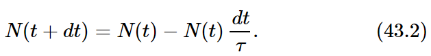
We shall find the answer to the general question: “What is the probability that a molecule will go for a time t without having a collision?” At some arbitrary instant—that we call t=0—we begin to watch a particular molecule. What is the chance that it gets by until t without colliding with another molecule? To compute the probability, we observe what is happening to all N0 molecules in a container. After we have waited a time t, some of them will have had collisions. We let N(t) be the number that have not had collisions up to the time t. N(t) is, of course, less than N0. We can find N(t) because we know how it changes with time. If we know that N(t) molecules have got by until t, then N(t+dt), the number which get by until t+dt, is less than N(t) by the number that have collisions in dt. The number that collide in dt we have written above in terms of the mean time τ as dN=N(t)dt/τ. We have the equation
The quantity on the left-hand side, N(t+dt), can be written, according to the definitions of calculus, as N(t)+(dN/dt)dt. Making this substitution, Eq. (43.2) yields
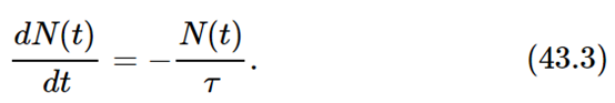
The number that are being lost in the interval dt is proportional to the number that are present, and inversely proportional to the mean life τ. Equation (43.3) is easily integrated if we rewrite it as
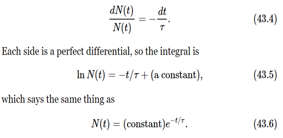
We know that the constant must be just N0, the total number of molecules present, since all of them start at t=0 to wait for their “next” collision. We can write our result as
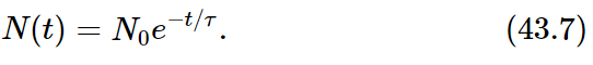
If we wish the probability of no collision, P(t), we can get it by dividing N(t) by N0, so
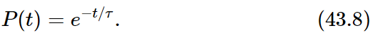
Our result is: the probability that a particular molecule survives a time t without a collision is e−t/τ, where τ is the mean time between collisions. The probability starts out at 1 (or certainty) for t=0, and gets less as t gets bigger and bigger. The probability that the molecule avoids a collision for a time equal to τ is e−1≈0.37. The chance is less than one-half that it will have a greater than average time between collisions. That is all right, because there are enough molecules which go collision-free for times much longer than the mean time before colliding, so that the average time can still be τ.
We originally defined τ as the average time between collisions. The result we have obtained in Eq. (43.7) also says that the mean time from an arbitrary starting instant to the next collision is also τ. We can demonstrate this somewhat surprising fact in the following way. The number of molecules which experience their next collision in the interval dt at the time t after an arbitrarily chosen starting time is N(t)dt/τ. Their “time until the next collision” is, of course, just t. The “average time until the next collision” is obtained in the usual way:

Using N(t) obtained in (43.7) and evaluating the integral, we find indeed that τ is the average time from any instant until the next collision.


|
|
|
|
التوتر والسرطان.. علماء يحذرون من "صلة خطيرة"
|
|
|
|
|
|
|
مرآة السيارة: مدى دقة عكسها للصورة الصحيحة
|
|
|
|
|
|
|
نحو شراكة وطنية متكاملة.. الأمين العام للعتبة الحسينية يبحث مع وكيل وزارة الخارجية آفاق التعاون المؤسسي
|
|
|