So far we have encountered

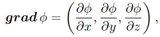 (1.1)

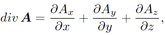
which is a vector field formed from a scalar field, and

 (1.2)

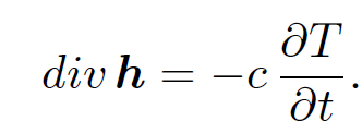
which is a scalar field formed from a vector field. There are two ways in which we can combine grad and div. We can either form the vector field grad(divA) or the scalar field div(grad ϕ). The former is not particularly interesting, but the scalar field div(grad ϕ) turns up in a great many physics problems and is, therefore, worthy of discussion. Let us introduce the heat flow vector h which is the rate of flow of heat energy per unit area across a surface perpendicular to the direction of h. In many substances heat flows directly down the temperature gradient, so that we can write

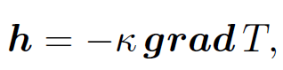 (1.3)

where is the thermal conductivity. The net rate of heat flow  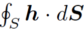out of some closed surface S must be equal to the rate of decrease of heat energy in the volume V enclosed by S. Thus, we can write

 (1.4)

where c is the specific heat. It follows from the divergence theorem that

 (1.5)

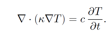
Taking the divergence of both sides of Eq. (1.3), and making use of Eq. (1.5), we obtain

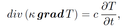 (1.6)

or

 (1.7)

If · is constant then the above equation can be written

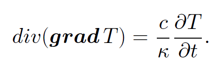 (1.8)

The scalar field div(grad T) takes the form

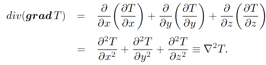 (1.9)

Here, the scalar differential operator

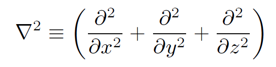 (1.10)

is called the Laplacian. The Laplacian is a good scalar operator (i.e., it is coordinate independent) because it is formed from a combination of div (another good scalar operator) and grad (a good vector operator). What is the physical significance of the Laplacian? In one-dimension ∇²T reduces to ∂²T/∂x². Now, ∂²T/∂x² is positive if T(x) is concave (from above)

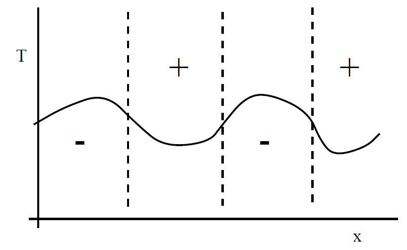
and negative if it is convex. So, if T is less than the average of T in its surroundings then ∇²T is positive, and vice versa. In two dimensions

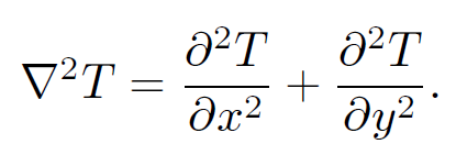 (1.11)

Consider a local minimum of the temperature. At the minimum the slope of T increases in all directions so ∇²T is positive. Likewise, ∇²T is negative at a local maximum. Consider, now, a steep-sided valley in T. Suppose that the bottom of the valley runs parallel to the x-axis. At the bottom of the valley ∂²T/∂y² is large and positive, whereas ∂²T/∂x² is small and may even be negative. Thus, ∇²T is positive, and this is associated with T being less than the average local value  Let us now return to the heat conduction problem:

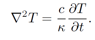 (1.12)

It is clear that if ∇²T is positive then T is locally less than the average value, so ∂T=∂t > 0; i.e., the region heats up. Likewise, if ∇²T is negative then T is locally greater than the average value and heat flows out of the region; i.e., ∂T=∂t < 0. Thus, the above heat conduction equation makes physical sense.

مواضيع ذات صلة

أصول عدم الانعكاس

الانعكاس يولد الانعكاس

الاحتمالية في الميكانيكا الإحصائية

القابلية للانعكاس وعدم القابلية للانعكاس

نظرة في تعددية الفيزياء

الاختزال وعدم القابلية للانعكاس

الواقعية العلمية وتغيير النظريات

نقص الإثبات ومذهب الذرائعية ومذهب الواقعية

مشكلة التمييز: متى يكون المنهج علميا؟

المنهج العلمي: من الاستقراء إلى التكذيب وما بعده

مناهج العلوم وثمارها

!Parity is not conserved