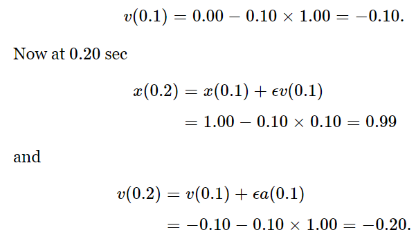
let us really solve the problem. Suppose that we take ϵ=0.100 sec. After we do all the work if we find that this is not small enough we may have to go back and do it again with ϵ=0.010 sec. Starting with our initial value x(0)=1.00, what is x(0.1)? It is the old position x(0) plus the velocity (which is zero) times 0.10 sec. Thus x(0.1) is still 1.00 because it has not yet started to move. But the new velocity at 0.10 sec will be the old velocity v(0)=0 plus ϵ times the acceleration. The acceleration is −x(0)=−1.00. Thus

And so, on and on and on, we can calculate the rest of the motion, and that is just what we shall do. However, for practical purposes there are some little tricks by which we can increase the accuracy. If we continued this calculation as we have started it, we would find the motion only rather crudely because ϵ=0.100 sec is rather crude, and we would have to go to a very small interval, say ϵ=0.01. Then to go through a reasonable total time interval would take a lot of cycles of computation. So we shall organize the work in a way that will increase the precision of our calculations, using the same coarse interval ϵ=0.10 sec. This can be done if we make a subtle improvement in the technique of the analysis.

Notice that the new position is the old position plus the time interval ϵ times the velocity. But the velocity when? The velocity at the beginning of the time interval is one velocity and the velocity at the end of the time interval is another velocity. Our improvement is to use the velocity halfway between. If we know the speed now, but the speed is changing, then we are not going to get the right answer by going at the same speed as now. We should use some speed between the “now” speed and the “then” speed at the end of the interval. The same considerations also apply to the velocity: to compute the velocity changes, we should use the acceleration midway between the two times at which the velocity is to be found. Thus, the equations that we shall actually use will be something like this: the position later is equal to the position before plus ϵ times the velocity at the time in the middle of the interval. Similarly, the velocity at this halfway point is the velocity at a time ϵ before (which is in the middle of the previous interval) plus ϵ times the acceleration at the time t. That is, we use the equations

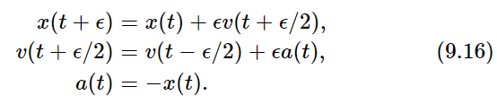
There remains only one slight problem: what is v(ϵ/2)? At the start, we are given v(0), not v(−ϵ/2). To get our calculation started, we shall use a special equation, namely, v(ϵ/2) = v(0) + (ϵ/2)a(0).

Table 9–1

Solution of dv_x/dt=−x

Interval: ϵ=0.10 sec

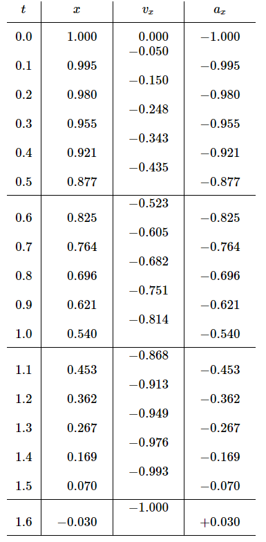
Now we are ready to carry through our calculation. For convenience, we may arrange the work in the form of a table, with columns for the time, the position, the velocity, and the acceleration, and the in-between lines for the velocity, as shown in Table 9–1. Such a table is, of course, just a convenient way of representing the numerical values obtained from the set of equations (9.16), and in fact the equations themselves need never be written. We just fill in the various spaces in the table one by one. This table now gives us a very good idea of the motion: it starts from rest, first picks up a little upward (negative) velocity and it loses some of its distance. The acceleration is then a little bit less but it is still gaining speed. But as it goes on it gains speed more and more slowly, until as it passes x=0 at about t=1.50 sec we can confidently predict that it will keep going, but now it will be on the other side; the position x will become negative, the acceleration therefore positive. Thus, the speed decreases. It is interesting to compare these numbers with the function x=cos t, which is done in Fig. 9–4. The agreement is within the three significant figure accuracy of our calculation! We shall see later that x=cos t is the exact mathematical solution of our equation of motion, but it is an impressive illustration of the power of numerical analysis that such an easy calculation should give such precise results.

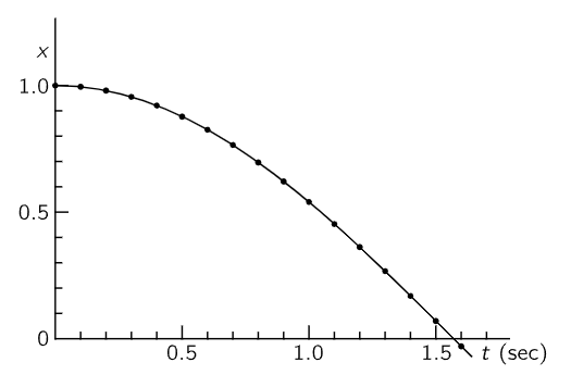
Fig. 9–4. Graph of the motion of a mass on a spring.

مواضيع ذات صلة

Reversibility in mechanics

The ratchet as an engine

How a ratchet works

The Doppler effect

Finding the “apparent” motion

Series and parallel impedances

Analogs in physics

Oscillations in linear systems

Damped oscillations

The energy of an oscillator

The forced oscillator with damping

Complex numbers and harmonic motion