Let us return now to the random walk and consider a modification of it. Suppose that in addition to a random choice of the direction (+ or −) of each step, the length of each step also varied in some unpredictable way, the only condition being that on the average the step length was one unit. This case is more representative of something like the thermal motion of a molecule in a gas. If we call the length of a step S, then S may have any value at all, but most often will be “near” 1. To be specific, we shall let ⟨S²⟩=1 or, equivalently, S_rms=1. Our derivation for ⟨D²⟩ would proceed as before except that Eq. (6.8) would be changed now to read

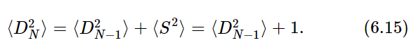
We have, as before, that

What would we expect now for the distribution of distances D? What is, for example, the probability that D=0 after 30 steps? The answer is zero! The probability is zero that D will be any particular value, since there is no chance at all that the sum of the backward steps (of varying lengths) would exactly equal the sum of forward steps. We cannot plot a graph like that of Fig. 6–2.

We can, however, obtain a representation similar to that of Fig. 6–2, if we ask, not what is the probability of obtaining D exactly equal to 0, 1, or 2, but instead what is the probability of obtaining D near 0, 1, or 2. Let us define P(x,Δx) as the probability that D will lie in the interval Δx located at x (say from x to x+Δx). We expect that for small Δx the chance of D landing in the interval is proportional to Δx, the width of the interval. So we can write

The function p(x) is called the probability density.

The form of p(x) will depend on N, the number of steps taken, and also on the distribution of individual step lengths. We cannot demonstrate the proofs here, but for large N, p(x) is the same for all reasonable distributions in individual step lengths, and depends only on N. We plot p(x) for three values of N in Fig. 6–7. You will notice that the “half-widths” (typical spread from x=0) of these curves is √N, as we have shown it should be.

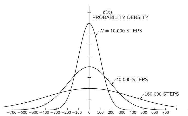
Fig. 6–7. The probability density for ending up at the distance D from the starting place in a random walk of N steps. (D is measured in units of the rms step length.)

You may notice also that the value of p(x) near zero is inversely proportional to √N. This comes about because the curves are all of a similar shape and their areas under the curves must all be equal. Since p(x)Δx is the probability of finding D in Δx when Δx is small, we can determine the chance of finding D somewhere inside an arbitrary interval from x₁ to x₂, by cutting the interval in a number of small increments Δx and evaluating the sum of the terms p(x)Δx for each increment. The probability that D lands somewhere between x₁ and x₂, which we may write P(x₁<D<x₂), is equal to the shaded area in Fig. 6–8. The smaller we take the increments Δx, the more correct is our result. We can write, therefore,

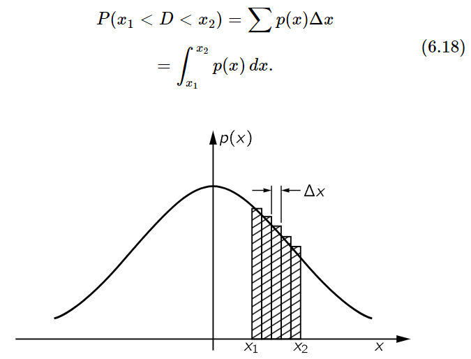
Fig. 6–8. The probability that the distance D traveled in a random walk is between x₁ and x₂ is the area under the curve of p(x) from x₁ to x₂.

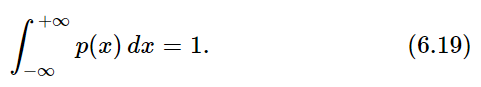
The area under the whole curve is the probability that D lands somewhere (that is, has some value between x=−∞ and x=+∞). That probability is surely 1. We must have that

Since the curves in Fig. 6–7 get wider in proportion to √N, their heights must be proportional to 1/√N to maintain the total area equal to 1.

The probability density function we have been describing is one that is encountered most commonly. It is known as the normal or Gaussian probability density. It has the mathematical form

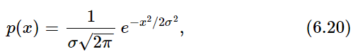
where σ is called the standard deviation and is given, in our case, by σ=√N or, if the rms step size is different from 1, by σ=√N S_rms.

We remarked earlier that the motion of a molecule, or of any particle, in a gas is like a random walk. Suppose we open a bottle of an organic compound and let some of its vapor escape into the air. If there are air currents, so that the air is circulating, the currents will also carry the vapor with them. But even in perfectly still air, the vapor will gradually spread out—will diffuse—until it has penetrated throughout the room. We might detect it by its color or odor. The individual molecules of the organic vapor spread out in still air because of the molecular motions caused by collisions with other molecules. If we know the average “step” size, and the number of steps taken per second, we can find the probability that one, or several, molecules will be found at some distance from their starting point after any particular passage of time. As time passes, more steps are taken and the gas spreads out as in the successive curves of Fig. 6–7. In a later chapter, we shall find out how the step sizes and step frequencies are related to the temperature and pressure of a gas.

Earlier, we said that the pressure of a gas is due to the molecules bouncing against the walls of the container. When we come later to make a more quantitative description, we will wish to know how fast the molecules are going when they bounce, since the impact they make will depend on that speed. We cannot, however, speak of the speed of the molecules. It is necessary to use a probability description. A molecule may have any speed, but some speeds are more likely than others. We describe what is going on by saying that the probability that any particular molecule will have a speed between v and v+Δv is p(v)Δv, where p(v), a probability density, is a given function of the speed v. We shall see later how Maxwell, using common sense and the ideas of probability, was able to find a mathematical expression for p(v). The form² of the function p(v) is shown in Fig. 6–9. Velocities may have any value, but are most likely to be near the most probable value v_p.

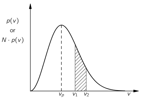
Fig. 6–9. The distribution of velocities of the molecules in a gas.

We often think of the curve of Fig. 6–9 in a somewhat different way. If we consider the molecules in a typical container (with a volume of, say, one liter), then there are a very large number N of molecules present (N≈10²²). Since p(v) Δv is the probability that one molecule will have its velocity in Δv, by our definition of probability we mean that the expected number ⟨ΔN⟩ to be found with a velocity in the interval Δv is given by

We call Np(v) the “distribution in velocity.” The area under the curve between two velocities v₁ and v₂, for example the shaded area in Fig. 6–9, represents [for the curve Np(v)] the expected number of molecules with velocities between v₁ and v₂. Since with a gas we are usually dealing with large numbers of molecules, we expect the deviations from the expected numbers to be small (like 1/√N), so we often neglect to say the “expected” number, and say instead: “The number of molecules with velocities between v₁ and v₂ is the area under the curve.” We should remember, however, that such statements are always about probable numbers.

_____________________________________
margin

2- Maxwell’s expression is p(v)=Cv²e−^{av^2}, where a is a constant related to the temperature and C is chosen so that the total probability is one.