The Distribution Function and the Fermi Energy

To begin to understand the meaning of the distribution function and the Fermi energy, we can plot the distribution function versus energy. Initially, let T = 0 K and consider the case when E < E_F. The exponential term in Equation (1) becomes exp[(E - E_F)/kT] → exp (-∞) = 0. The resulting distribution function is f_F(E < E_F) = 1 . Again let T = 0 K and consider the case when E > E_F. The exponential term in the distribution function becomes exp[(E - E_F)/kT] → exp (+∞) → + ∞. The resulting Fermi-Dirac distribution function now becomes f_F(E > E_F) = 0.

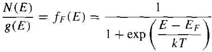(1)

The Fermi-Dirac distribution function for T = 0 K is plotted in Figure 1.1. This result shows that, for T = 0 K, the electrons are in their lowest possible energy states. The probability of a quantum state being occupied is unity for E < E_F and the probability of a state being occupied is zero for E > E_F. All electrons have energies below the Fermi energy at T = 0 K.

Figure 1.2 shows discrete energy levels of a particular system as well as the number of available quantum states at each energy. If we assume, for this case, that

Figure 1.1 The Fermi probability function versus energy for T = 0 K.

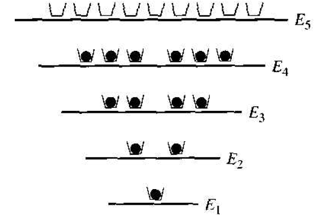
Figure 1.2 Discrete energy states and quantum states for a particular system at T = 0 K.

the system contains 13 electrons, then Figure 1.2 shows how these electrons are distributed among the various quantum states at T = 0 K. The electrons will be in the lowest possible energy state, so the probability of a quantum state being occupied in energy levels E₁ through E₄ is unity, and the probability of a quantum state being occupied in energy level E₅ is zero. The Fermi energy, for this case, must be above E₄ but less than E₅. The Fermi energy determines the statistical distribution of electrons and does not have to correspond to an allowed energy level.

Now consider a case in which the density of quantum states g(E) is a continuous function of energy as shown in Figure 1.3. If we have N₀ electrons in this system, then the distribution of these electrons among the quantum states at T = 0 K is shown by the dashed line. The electrons are in the lowest possible energy state so that all states below EF are tilled and all states above EF are empty. If g(E) and N₀ are known for this particular system, then the Fermi energy E_F can be determined.

Consider the situation when the temperature increases above T = 0 K. Electrons gain a certain amount of thermal energy so that some electrons can jump to higher energy levels, which means that the distribution of electrons among the available energy states will change. Figure 1.4 shows the same discrete energy levels. The distribution of electrons among the quantum states has changed from the T = 0 K case. Two electrons from the E₄ level have gained enough energy to jump to E₅, and one electron from E₃ has jumped to E₄. As the temperature changes, the distribution of electrons versus energy changes.

The change in the electron distribution among energy levels for T > 0 K can be seen by plotting the Fermi-Dirac distribution function. If we let E = E_F and T > 0 K, then Equation (1) becomes

The probability of a state being occupied at E = E_F is 1/2. Figure 1.5 shows the Fermi-Dirac distribution function plotted for several temperatures, assuming the Fermi energy is independent of temperature.

Figure 1.3 Density of quantum states and electrons in a continuous energy system at T = 0 K.

Figure 1.4 Discrete energy states and quantum states for the same system shown in Figure 1.2 for T > 0 K.

Figure 1.5 The Fermi probability function versus energy for different temperatures.

We can see that for temperatures above absolute zero, there is a nonzero probability that some energy states above E_F will be occupied by electrons and some energy states below E_F will be empty. This result again means that some electrons have jumped to higher energy levels with increasing thermal energy.

We can see from Figure 1.5 that the probability of an energy above E_F being occupied increases as the temperature increases and the probability of a state below E_F being empty increases as the temperature increases.

We may note that the probability of a state a distance dE above E_F being occupied is the same as the probability of a state a distance dE below E_F empty. The function f_F (E) is symmetrical with the function 1 – f_F (E) about the Fermi energy, E_F. This symmetry effect is shown in Figure 1.6 and will be us in the next chapter.

Figure 1.6 The probability of a slate being occupied. f_F(E), and the probability of a state being empty, 1 - f_F(E).

Figure 1.7 The Fermi-Dirac probability function and the Maxwell-Boltzmann approximation.

Consider the case when E - E_F >> kT. where the exponential term in the denominator of Equation (1) is much greater than unity. We may neglect the 1 in the denominator, so the Femi-Dirac distribution function becomes

(2)

Equation (2) is known as the Maxwell-Boltzmann approximation, or simply the Boltzmann approximation. to the Fermi-Dirac distribution function. Figure 1.7 shows the Femi-Dirac probability function and the Boltzmann approximation. This figure gives an indication of the range of energies over which the approximation is valid.

مواضيع ذات صلة

أنظمة لأكثر من جسيم واحد

كمية التحرك الزاوية والقوة المركزية

الحركة الدورانية

امثلة عن الاتزان الاستاتيكي للأجسام الممتدة

الاتزان الاستاتيكي للأجسام الممتدة

تعريف العزم

تذبذبات صغيرة لبندول

اعتبارات الطاقة في الحركة التوافقية البسيطة

الحل الهندسي للمعادلة التفاضلية للحركة التوافقية البسيطة، دائرة المرجع

الحل باستخدام حساب التفاضل والتكامل

قانون هوك والمعادلة التفاضلية للحركة التوافقية البسيطة

القدرة ووحدات الشغل