We shall now discuss a few of the ideas associated with potential energy and with the idea of a field. Suppose we have two large objects A and B and a third very small one which is attracted gravitationally by the two, with some resultant force F. The gravitational force on a particle can be written as its mass, m, times another vector, C, which is dependent only upon the position of the particle:

F=mC.

We can analyze gravitation, then, by imagining that there is a certain vector C at every position in space which “acts” upon a mass which we may place there, but which is there itself whether we actually supply a mass for it to “act” on or not. C has three components, and each of those components is a function of (x,y,z), a function of position in space. Such a thing we call a field, and we say that the objects A and B generate the field, i.e., they “make” the vector C. When an object is put in a field, the force on it is equal to its mass times the value of the field vector at the point where the object is put.

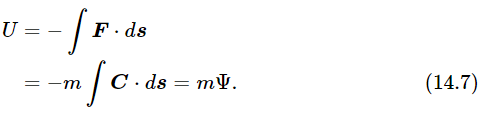
We can also do the same with the potential energy. Since the potential energy, the integral of (−force)⋅(ds) can be written as m times the integral of (−field)⋅(ds), a mere change of scale, we see that the potential energy U(x,y,z) of an object located at a point (x,y,z) in space can be written as m times another function which we may call the potential Ψ. The integral ∫C⋅ds=−Ψ, just as ∫F⋅ds=−U; there is only a scale factor between the two:

By having this function Ψ(x,y,z) at every point in space, we can immediately calculate the potential energy of an object at any point in space, namely, U(x,y,z)=mΨ(x,y,z)—rather a trivial business, it seems. But it is not really trivial, because it is sometimes much nicer to describe the field by giving the value of Ψ everywhere in space instead of having to give C. Instead of having to write three complicated components of a vector function, we can give instead the scalar function Ψ. Furthermore, it is much easier to calculate Ψ than any given component of C when the field is produced by a number of masses, for since the potential is a scalar we merely add, without worrying about direction. Also, the field C can be recovered easily from Ψ, as we shall shortly see. Suppose we have point masses m₁, m₂, … at the points 1, 2, … and we wish to know the potential Ψ at some arbitrary point p. This is simply the sum of the potentials at p due to the individual masses taken one by one:

Fig. 14–4. Potential due to a spherical shell of radius a.

We used this formula, that the potential is the sum of the potentials from all the different objects, to calculate the potential due to a spherical shell of matter by adding the contributions to the potential at a point from all parts of the shell. The result of this calculation is shown graphically in Fig. 14–4. It is negative, having the value zero at r=∞ and varying as 1/r down to the radius a, and then is constant inside the shell. Outside the shell the potential is −Gm/r, where m is the mass of the shell, which is exactly the same as it would have been if all the mass were located at the center. But it is not everywhere exactly the same, for inside the shell the potential turns out to be −Gm/a, and is a constant! When the potential is constant, there is no field, or when the potential energy is constant there is no force, because if we move an object from one place to another anywhere inside the sphere the work done by the force is exactly zero. Why? Because the work done in moving the object from one place to the other is equal to minus the change in the potential energy (or, the corresponding field integral is the change of the potential). But the potential energy is the same at any two points inside, so there is zero change in potential energy, and therefore no work is done in going between any two points inside the shell. The only way the work can be zero for all directions of displacement is that there is no force at all.

This gives us a clue as to how we can obtain the force or the field, given the potential energy. Let us suppose that the potential energy of an object is known at the position (x,y,z) and we want to know what the force on the object is. It will not do to know the potential at only this one point, as we shall see; it requires knowledge of the potential at neighboring points as well. Why? How can we calculate the x–component of the force? (If we can do this, of course, we can also find the y– and z–components, and we will then know the whole force.) Now, if we were to move the object a small distance Δx, the work done by the force on the object would be the x–component of the force times Δx, if Δx is sufficiently small, and this should equal the change in potential energy in going from one point to the other:

We have merely used the formula ∫F⋅ds=−ΔU, but for a very short path. Now we divide by Δx and so find that the force is

Of course, this is not exact. What we really want is the limit of (14.10) as Δx gets smaller and smaller, because it is only exactly right in the limit of infinitesimal Δx. This we recognize as the derivative of U with respect to x, and we would be inclined, therefore, to write −dU/dx. But U depends on x, y, and z, and the mathematicians have invented a different symbol to remind us to be very careful when we are differentiating such a function, so as to remember that we are considering that only x varies, and y and z do not vary. Instead of a d they simply make a “backwards 6,” or ∂. (A ∂ should have been used in the beginning of calculus because we always want to cancel that d, but we never want to cancel a ∂!) So they write ∂U/∂x, and furthermore, in moments of duress, if they want to be very careful, they put a line beside it with a little yz at the bottom (∂U/∂x|_yz), which means “Take the derivative of U with respect to x, keeping y and z constant.” Most often we leave out the remark about what is kept constant because it is usually evident from the context, so we usually do not use the line with the y and z. However, always use a ∂ instead of a d as a warning that it is a derivative with some other variables kept constant. This is called a partial derivative; it is a derivative in which we vary only x.

Therefore, we find that the force in the x–direction is minus the partial derivative of U with respect to x:

In a similar way, the force in the y–direction can be found by differentiating U with respect to y, keeping x and z constant, and the third component, of course, is the derivative with respect to z, keeping y and x constant:

This is the way to get from the potential energy to the force. We get the field from the potential in exactly the same way:

Incidentally, we shall mention here another notation, which we shall not actually use for quite a while: Since C is a vector and has x–, y–, and z–components, the symbolized ∂/∂x, ∂/∂y, and ∂/∂z which produce the x–, y–, and z–components are something like vectors. The mathematicians have invented a glorious new symbol, ∇, called “grad” or “gradient”, which is not a quantity but an operator that makes a vector from a scalar. It has the following “components”: The x–component of this “grad” is ∂/∂x, the y–component is ∂/∂y, and the z–component is ∂/∂z, and then we have the fun of writing our formulas this way:

Using ∇ gives us a quick way of testing whether we have a real vector equation or not, but actually Eqs. (14.14) mean precisely the same as Eqs. (14.11), (14.12) and (14.13); it is just another way of writing them, and since we do not want to write three equations every time, we just write ∇U instead.

One more example of fields and potentials has to do with the electrical case. In the case of electricity, the force on a stationary object is the charge times the electric field: F=qE. (In general, of course, the x–component of force in an electrical problem has also a part which depends on the magnetic field. It is easy to show from Eq. (12.11) that the force on a particle due to magnetic fields is always at right angles to its velocity, and also at right angles to the field. Since the force due to magnetism on a moving charge is at right angles to the velocity, no work is done by the magnetism on the moving charge because the motion is at right angles to the force. Therefore, in calculating theorems of kinetic energy in electric and magnetic fields we can disregard the contribution from the magnetic field, since it does not change the kinetic energy.) We suppose that there is only an electric field. Then we can calculate the energy, or work done, in the same way as for gravity, and calculate a quantity ϕ which is minus the integral of E⋅ds, from the arbitrary fixed point to the point where we make the calculation, and then the potential energy in an electric field is just charge times this quantity ϕ:

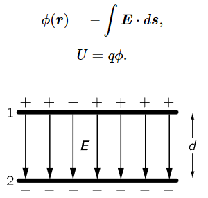
Fig. 14–5. Field between parallel plates.

Let us take, as an example, the case of two parallel metal plates, each with a surface charge of ±σ per unit area. This is called a parallel–plate capacitor. We found previously that there is zero force outside the plates and that there is a constant electric field between them, directed from + to − and of magnitude σ/ϵ₀ (Fig. 14–5). We would like to know how much work would be done in carrying a charge from one plate to the other. The work would be the (force)⋅(ds) integral, which can be written as charge times the potential value at plate 1 minus that at plate 2:

We can actually work out the integral because the force is constant, and if we call the separation of the plates d, then the integral is easy:

The difference in potential, Δϕ=σd/ϵ₀, is called the voltage difference, and ϕ is measured in volts. When we say a pair of plates is charged to a certain voltage, what we mean is that the difference in electrical potential of the two plates is so–and–so many volts. For a capacitor made of two parallel plates carrying a surface charge ±σ, the voltage, or difference in potential, of the pair of plates is σd/ϵ₀.

مواضيع ذات صلة

The Doppler effect

Finding the “apparent” motion

Series and parallel impedances

Analogs in physics

Oscillations in linear systems

Damped oscillations

The energy of an oscillator

The forced oscillator with damping

Complex numbers and harmonic motion

Forced oscillations

Initial conditions for Harmonic motion and circular motion

Harmonic motion and circular motion