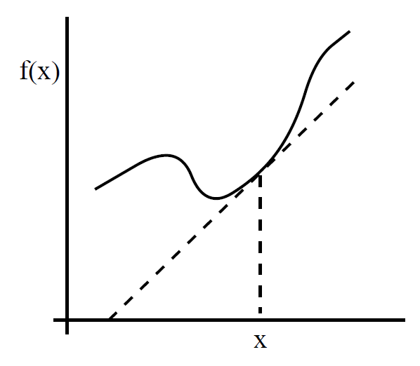
A one-dimensional function f(x) has a gradient df/dx which is defined as the slope of the tangent to the curve at x. We wish to extend this idea to cover scalar

fields in two and three dimensions. Consider a two-dimensional scalar field h(x, y) which is (say) the height of a hill. Let dl = (dx, dy) be an element of horizontal distance. Consider dh/dl, where dh is the change in height after moving an infinitesimal distance dl. This quantity is somewhat like the one-dimensional gradient, except that dh depends on the direction of dl, as well as its magnitude. In the immediate vicinity of some

point P the slope reduces to an inclined plane. The largest value of dh/dl is straight up the slope. For any other direction

 (1.1)

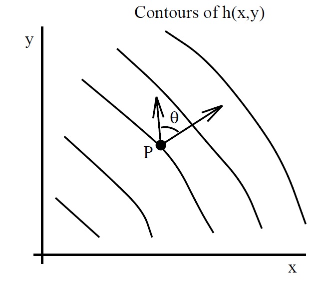
Let us define a two-dimensional vector grad h, called the gradient of h, whose magnitude is (dh/dl)max and whose direction is the direction of the steepest slope. Because of the cos θ property, the component of grad h in any direction equals dh/dl for that direction. The component of dh/dl in the x-direction can be obtained by plotting out the profile of h at constant y, and then finding the slope of the tangent to the curve at given x. This quantity is known as the partial derivative of h with respect to x at constant y, and is denoted (∂h/∂x)y. Likewise, the gradient of the profile at constant x is written (∂h/∂y)x. Note that the subscripts denoting constant-x and constant-y are usually omitted, unless there is any ambiguity. If follows that in component form

 (1.2)

Now, the equation of the tangent plane at P = (x₀, y₀) is

 (1.3)

This has the same local gradients as h(x, y), so

   (1.4)

by differentiation of the above. For small dx = x-x₀ and dy = y-y₀ the function h is coincident with the tangent plane. We have

 (1.5)

but grad h = (∂h/∂x, ∂h/∂y) and dl = (dx, dy), so

  (1.6)

Incidentally, the above equation demonstrates that grad h is a proper vector, since the left-hand side is a scalar and, according to the properties of the dot product, the right-hand side is also a scalar provided that dl and grad h are both proper vectors (dl is an obvious vector because it is directly derived from displacements). Consider, now, a three-dimensional temperature distribution T(x, y, z) in (say) a reaction vessel. Let us define grad T, as before, as a vector whose magnitude is (dT/dl)max and whose direction is the direction of the maximum gradient. This vector is written in component form

 (1.7)

Here, ∂T/∂x ≡ (∂T/∂x)_y,z is the gradient of the one-dimensional temperature profile at constant y and z. The change in T in going from point P to a neigh-bouring point offset by dl = (dx, dy, dz) is

 (1.8)

In vector form this becomes

 (1.9)

Suppose that dT = 0 for some dl. It follows that

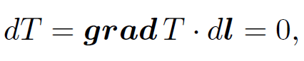 (1.10)

so dl is perpendicular to grad T. Since dT = 0 along so-called ''isotherms" (i.e., contours of the temperature) we conclude that the isotherms (contours) are everywhere perpendicular to grad T.

It is, of course, possible to integrate dT . The line integral from point P to point Q is written

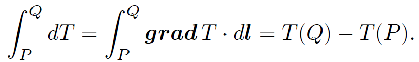 (1.11)

This integral is clearly independent of the path taken between P and Q, so  grad T . dl must be path independent. In general,  A . dl depends on path, but for some special vector fields the integral is path independent. Such fields are called conservative fields. It can be shown that if A is a conservative field then A = grad ϕ for some scalar field ϕ. The proof of this is straightforward. Keeping P fixed we have

 (1.12)

where V (Q) is a well-defined function due to the path independent nature of the line integral. Consider moving the position of the end point by an infinitesimal amount dx in the x-direction. We have

 (1.13)

Hence,

 (1.14)

with analogous relations for the other components of A. It follows that

 (1.15)

In physics, the force due to gravity is a good example of a conservative field. If A is a force, then ∫A . dl is the work done in traversing some path. If A is conservative then

 (1.16)

where corresponds to the line integral around some closed loop. The fact that zero net work is done in going around a closed loop is equivalent to the conservation of energy (this is why conservative fields are called ''conservative"). A good example of a non-conservative field is the force due to friction. Clearly, a frictional system loses energy in going around a closed cycle, so

.

It is useful to define the vector operator

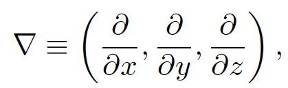 (1.17)

which is usually called the ''grad" or ''del" operator. This operator acts on everything to its right in a expression until the end of the expression or a closing bracket is reached. For instance,

 (1.18)

For two scalar fields ϕ and ψ,

 (1.19)

can be written more succinctly as

 (1.20)

Suppose that we rotate the basis about the z-axis by µ degrees. By analogy the old coordinates (x, y, z) are related to the new ones (xʹ, yʹ, zʹ) via

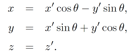 (1.21)

Now,

 (1.22)

giving

 (1.23)

and

 (1.24)

It can be seen that the differential operator ∇ transforms like a proper vector. This is another proof that ∇f is a good vector.

مواضيع ذات صلة

أصول عدم الانعكاس

الانعكاس يولد الانعكاس

الاحتمالية في الميكانيكا الإحصائية

القابلية للانعكاس وعدم القابلية للانعكاس

نظرة في تعددية الفيزياء

الاختزال وعدم القابلية للانعكاس

الواقعية العلمية وتغيير النظريات

نقص الإثبات ومذهب الذرائعية ومذهب الواقعية

مشكلة التمييز: متى يكون المنهج علميا؟

المنهج العلمي: من الاستقراء إلى التكذيب وما بعده

مناهج العلوم وثمارها

!Parity is not conserved