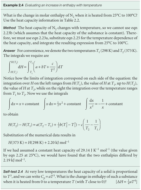
The variation of enthalpy with temperature
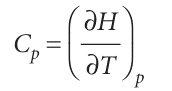
The enthalpy of a substance increases as its temperature is raised. The relation between the increase in enthalpy and the increase in temperature depends on the conditions (for example, constant pressure or constant volume). The most important condition is constant pressure, and the slope of the tangent to a plot of enthalpy against temperature at constant pressure is called the heat capacity at constant pressure, Cp, at a given temperature (Fig. 2.14). More formally:
The heat capacity at constant pressure is the analogue of the heat capacity at constant volume, and is an extensive property.4 The molar heat capacity at constant pressure, Cp, m, is the heat capacity per mole of material; it is an intensive property. The heat capacity at constant pressure is used to relate the change in enthalpy to a change in temperature. For infinitesimal changes of temperature, dH=CpdT (at constant pressure) If the heat capacity is constant over the range of temperatures of interest, then for a measurable increase in temperature , ∆H=Cp∆T (at constant pressure) , Because an increase in enthalpy can be equated with the energy supplied as heat at constant pressure, the practical form of the latter equation is , qp =Cp∆T , This expression shows us how to measure the heat capacity of a sample: a measured quantity of energy is supplied as heat under conditions of constant pressure (as in a sample exposed to the atmosphere and free to expand), and the temperature rise is monitored. The variation of heat capacity with temperature can sometimes be ignored if the temperature range is small; this approximation is highly accurate for a monatomic perfect gas (for instance, one of the noble gases at low pressure). However, when it is necessary to take the variation into account, a convenient approximate empirical expression is
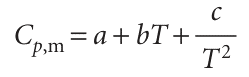
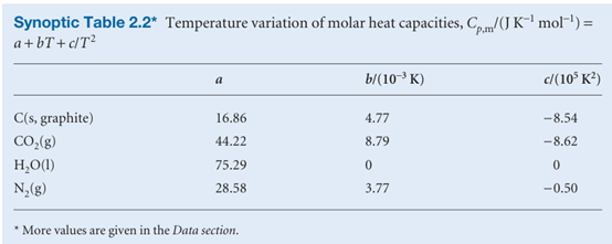
The empirical parameters a, b, and c are independent of temperature (Table 2.2).
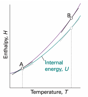
Fig. 2.14 The slope of the tangent to a curve of the enthalpy of a system subjected to a constant pressure plotted against temperature is the constant-pressure heat capacity. The slope may change with temperature, in which case the heat capacity varies with temperature. Thus, the heat capacities at A and B are different. For gases, at a given temperature the slope of enthalpy versus temperature is steeper than that of internal energy versus temperature, and Cp,m is larger than CV, m.
Most systems expand when heated at constant pressure. Such systems do work on the surroundings and therefore some of the energy supplied to them as heat escapes back to the surroundings. As a result, the temperature of the system rises less than when the heating occurs at constant volume. A smaller increase in temperature implies a larger heat capacity, so we conclude that in most cases the heat capacity at constant pressure of a system is larger than its heat capacity at constant volume. We show later (Section 2.11) that there is a simple relation between the two heat capacities of a perfect gas: Cp −CV=nR , It follows that the molar heat capacity of a perfect gas is about 8 J K−1 mol−1 larger at constant pressure than at constant volume. Because the heat capacity at constant volume of a monatomic gas is about 12 J K−1 mol−1, the difference is highly significant and must be taken into account.
Adifferential scanning calorimeter (DSC) measures the energy transferred as heat to or from a sample at constant pressure during a physical or chemical change. The term ‘differential’ refers to the fact that the behaviour of the sample is compared to that of a reference material which does not undergo a physical or chemical change during the analysis. The term ‘scanning’ refers to the fact that the temperatures of the sample and reference material are increased, or scanned, during the analysis. A DSC consists of two small compartments that are heated electrically at a constant rate. The temperature, T, at time t during a linear scan is T = T0 + αt, where T0 is the initial temperature and α is the temperature scan rate (in kelvin per second, K s−1). A computer controls the electrical power output in order to maintain the same temperature in the sample and reference compartments throughout the analysis (see Fig. 2.15). The temperature of the sample changes significantly relative to that of the reference material if a chemical or physical process involving the transfer of energy as heat occurs in the sample during the scan. To maintain the same temperature in both compartments, excess energy is transferred as heat to or from the sample during the process. For example, an endothermic process lowers the temperature of the sample relative to that of the reference and, as a result, the sample must be heated more strongly than the reference in order to maintain equal temperatures. If no physical or chemical change occurs in the sample at temperature T, we write the heat transferred to the sample as qp = Cp∆T, where ∆T = T − T0 and we have assumed that Cp is independent of temperature. The chemical or physical process requires the transfer of qp + qp, ex, where qp, ex is excess energy transferred as heat, to attain the same change in temperature of the sample. We interpret qp, ex in terms of an apparent change in the heat capacity at constant pressure of the sample, Cp, during the temperature scan. Then we write the heat capacity of the sample as Cp + Cp, ex, and
qp +qp, ex = (Cp + Cp, ex) ∆T
It follows that
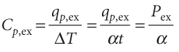
where Pex = qp, ex/t is the excess electrical power necessary to equalize the temperature of the sample and reference compartments. A DSC trace, also called a thermogram, consists of a plot of Pex or Cp, ex against T (see Fig. 2.16). Broad peaks in the thermogram indicate processes requiring transfer of energy as heat. From eqn 2.23a, the enthalpy change associated with the process is
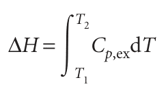
where T1 and T2 are, respectively, the temperatures at which the process begins and ends. This relation shows that the enthalpy change is then the area under the curve of Cp, ex against T. With a DSC, enthalpy changes may be determined in samples of masses as low as 0.5 mg, which is a significant advantage over bomb or flame calorimeters, which require several grams of material. Differential scanning calorimetry is used in the chemical industry to characterize polymers and in the biochemistry laboratory to assess the stability of proteins, nucleic acids, and membranes. Large molecules, such as synthetic or biological polymers, attain complex three-dimensional structures due to intra- and intermolecular inter actions, such as hydrogen bonding and hydrophobic interactions (Chapter 18). Disruption of these interactions is an endothermic process that can be studied with a DSC. For example, the thermogram shown in the illustration indicated that the pro tein ubiquitin retains its native structure up to about 45°C. At higher temperatures, the protein undergoes an endothermic conformational change that results in the loss of its three-dimensional structure. The same principles also apply to the study of structural integrity and stability of synthetic polymers, such as plastics.
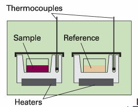
Fig. 2.15 A differential scanning calorimeter. The sample and a reference material are heated in separate but identical metal heat sinks. The output is the difference in power needed to maintain the heat sinks at equal temperatures as the temperature rises.
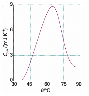
Fig. 2.16 A thermogram for the protein ubiquitin at pH = 2.45. The protein retains its native structure up to about 45oC and then undergoes an endothermic conformational change. (Adapted from B. Chowdhry and S. LeHarne, J. Chem. Educ. 74, 236 (1997).)


