تاريخ الفيزياء
علماء الفيزياء


الفيزياء الكلاسيكية
الميكانيك
الديناميكا الحرارية
الكهربائية والمغناطيسية
الكهربائية
المغناطيسية
الكهرومغناطيسية
علم البصريات
تاريخ علم البصريات
الضوء
مواضيع عامة في علم البصريات
الصوت
الفيزياء الحديثة
النظرية النسبية
النظرية النسبية الخاصة
النظرية النسبية العامة
مواضيع عامة في النظرية النسبية
ميكانيكا الكم
الفيزياء الذرية
الفيزياء الجزيئية
الفيزياء النووية
مواضيع عامة في الفيزياء النووية
النشاط الاشعاعي
فيزياء الحالة الصلبة
الموصلات
أشباه الموصلات
العوازل
مواضيع عامة في الفيزياء الصلبة
فيزياء الجوامد
الليزر
أنواع الليزر
بعض تطبيقات الليزر
مواضيع عامة في الليزر
علم الفلك
تاريخ وعلماء علم الفلك
الثقوب السوداء
المجموعة الشمسية
الشمس
كوكب عطارد
كوكب الزهرة
كوكب الأرض
كوكب المريخ
كوكب المشتري
كوكب زحل
كوكب أورانوس
كوكب نبتون
كوكب بلوتو
القمر
كواكب ومواضيع اخرى
مواضيع عامة في علم الفلك
النجوم
البلازما
الألكترونيات
خواص المادة
الطاقة البديلة
الطاقة الشمسية
مواضيع عامة في الطاقة البديلة
المد والجزر
فيزياء الجسيمات
الفيزياء والعلوم الأخرى
الفيزياء الكيميائية
الفيزياء الرياضية
الفيزياء الحيوية
الفيزياء والفلسفة
الفيزياء العامة
مواضيع عامة في الفيزياء
تجارب فيزيائية
مصطلحات وتعاريف فيزيائية
وحدات القياس الفيزيائية
طرائف الفيزياء
مواضيع اخرى

Molecular diffusion
 المؤلف:
Richard Feynman, Robert Leighton and Matthew Sands
المؤلف:
Richard Feynman, Robert Leighton and Matthew Sands
 المصدر:
The Feynman Lectures on Physics
المصدر:
The Feynman Lectures on Physics
 الجزء والصفحة:
Volume I, Chapter 43
الجزء والصفحة:
Volume I, Chapter 43
 2024-06-06
 2184
2184


+
-
20
We turn now to a different kind of problem, and a different kind of analysis: the theory of diffusion. Suppose that we have a container of gas in thermal equilibrium, and that we introduce a small amount of a different kind of gas at some place in the container. We shall call the original gas the “background” gas and the new one the “special” gas. The special gas will start to spread out through the whole container, but it will spread slowly because of the presence of the background gas. This slow spreading-out process is called diffusion. The diffusion is controlled mainly by the molecules of the special gas getting knocked about by the molecules of the background gas. After a large number of collisions, the special molecules end up spread out more or less evenly throughout the whole volume. We must be careful not to confuse diffusion of a gas with the gross transport that may occur due to convection currents. Most commonly, the mixing of two gases occurs by a combination of convection and diffusion. We are interested now only in the case that there are no “wind” currents. The gas is spreading only by molecular motions, by diffusion. We wish to compute how fast diffusion takes place.
We now compute the net flow of molecules of the “special” gas due to the molecular motions. There will be a net flow only when there is some nonuniform distribution of the molecules, otherwise all of the molecular motions would average to give no net flow. Let us consider first the flow in the x-direction. To find the flow, we consider an imaginary plane surface perpendicular to the x-axis and count the number of special molecules that cross this plane. To obtain the net flow, we must count as positive those molecules which cross in the direction of positive x and subtract from this number the number which cross in the negative x-direction. As we have seen many times, the number which cross a surface area in a time ΔT is given by the number which start the interval ΔT in a volume which extends the distance vΔT from the plane. (Note that v, here, is the actual molecular velocity, not the drift velocity.)
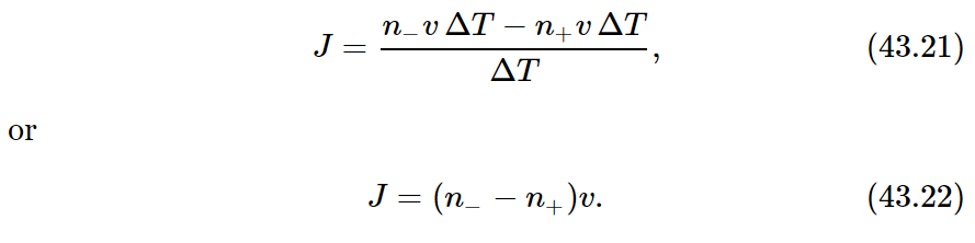
We shall simplify our algebra by giving our surface one unit of area. Then the number of special molecules which pass from left to right (taking the +x-direction to the right) is n−vΔT, where n− is the number of special molecules per unit volume to the left (within a factor of 2 or so, but we are ignoring such factors!). The number which cross from right to left is, similarly, n+vΔT, where n+ is the number density of special molecules on the right-hand side of the plane. If we call the molecular current J, by which we mean the net flow of molecules per unit area per unit time, we have
What shall we use for n− and n+? When we say “the density on the left,” how far to the left do we mean? We should choose the density at the place from which the molecules started their “flight,” because the number which start such trips is determined by the number present at that place. So by n− we should mean the density a distance to the left equal to the mean free path l, and by n+, the density at the distance l to the right of our imaginary surface.
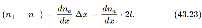
It is convenient to consider that the distribution of our special molecules in space is described by a continuous function of x, y, and z which we shall call na. By na(x,y,z) we mean the number density of special molecules in a small volume element centered on (x,y,z). In terms of na we can express the difference (n+− n−) as
Substituting this result in Eq. (43.22) and neglecting the factor of 2, we get
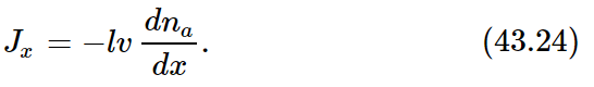
We have found that the flow of special molecules is proportional to the derivative of the density, or to what is sometimes called the “gradient” of the density.
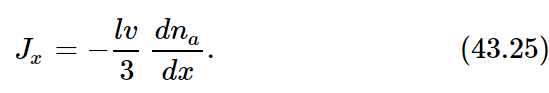
It is clear that we have made several rough approximations. Besides various factors of two we have left out, we have used v where we should have used vx, and we have assumed that n+ and n− refer to places at the perpendicular distance l from our surface, whereas for those molecules which do not travel perpendicular to the surface element, l should correspond to the slant distance from the surface. All of these refinements can be made; the result of a more careful analysis shows that the right-hand side of Eq. (43.24) should be multiplied by 1/3. So a better answer is
Similar equations can be written for the currents in the y- and z-directions.
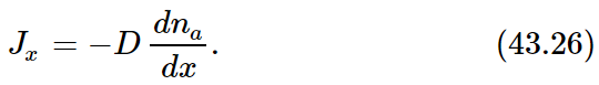
The current Jx and the density gradient dna/dx can be measured by macroscopic observations. Their experimentally determined ratio is called the “diffusion coefficient,” D. That is,
We have been able to show that for a gas we expect
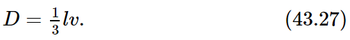
we have considered two distinct processes: mobility, the drift of molecules due to “outside” forces; and diffusion, the spreading determined only by the internal forces, the random collisions. There is, however, a relation between them, since they both depend basically on the thermal motions, and the mean free path l appears in both calculations.
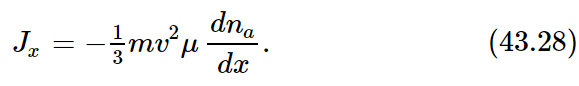
If, in Eq. (43.25), we substitute l=vτ and τ=μm, we have
But mv2 depends only on the temperature. We recall that
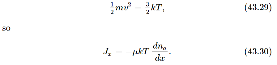
We find that D, the diffusion coefficient, is just kT times μ, the mobility coefficient:
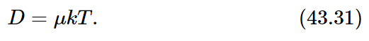
And it turns out that the numerical coefficient in (43.31) is exactly right—no extra factors have to be thrown in to adjust for our rough assumptions. We can show, in fact, that (43.31) must always be correct—even in complicated situations (for example, the case of a suspension in a liquid) where the details of our simple calculations would not apply at all.
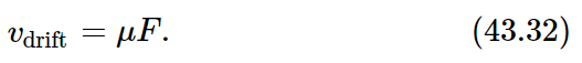
To show that (43.31) must be correct in general, we shall derive it in a different way, using only our basic principles of statistical mechanics. Imagine a situation in which there is a gradient of “special” molecules, and we have a diffusion current proportional to the density gradient, according to Eq. (43.26). We now apply a force field in the x-direction, so that each special molecule feels the force F. According to the definition of the mobility μ there will be a drift velocity given by
By our usual arguments, the drift current (the net number of molecules which pass a unit of area in a unit of time) will be
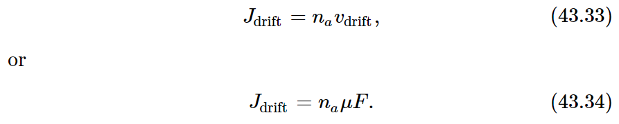
We now adjust the force F so that the drift current due to F just balances the diffusion, so that there is no net flow of our special molecules. We have Jx+Jdrift=0, or
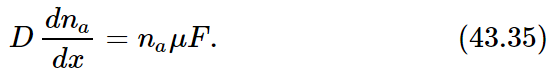
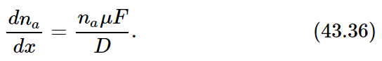
Under the “balance” conditions we find a steady (with time) gradient of density given by
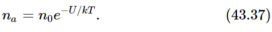
But notice! We are describing an equilibrium condition, so our equilibrium laws of statistical mechanics apply. According to these laws the probability of finding a molecule at the coordinate x is proportional to e−U/kT, where U is the potential energy. In terms of the number density na, this means that
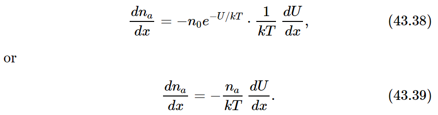
If we differentiate (43.37) with respect to x, we find
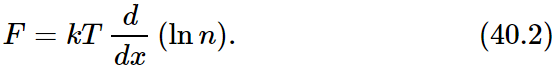
In our situation, since the force F is in the x-direction, the potential energy U is just −Fx, and −dU/dx=F. Equation (43.39) then gives
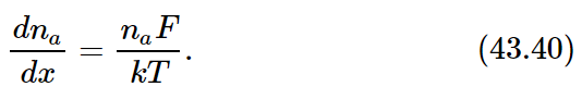
[This is just exactly Eq. (40.2), from which we deduced e−U/kT in the first place, so we have come in a circle].
Comparing (43.40) with (43.36), we get exactly Eq. (43.31). We have shown that Eq. (43.31), which gives the diffusion current in terms of the mobility, has the correct coefficient and is very generally true. Mobility and diffusion are intimately connected. This relation was first deduced by Einstein.
 الاكثر قراءة في الكهربائية
 اخر الاخبار
اخبار العتبة العباسية المقدسة

الآخبار الصحية


مواضيع ذات صلة
 قسم الشؤون الفكرية يصدر كتاباً يوثق تاريخ السدانة في العتبة العباسية المقدسة
 "المهمة".. إصدار قصصي يوثّق القصص الفائزة في مسابقة فتوى الدفاع المقدسة للقصة القصيرة
 (نوافذ).. إصدار أدبي يوثق القصص الفائزة في مسابقة الإمام العسكري (عليه السلام)