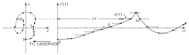
Fig. 34–2. A geometrical solution of Eq. (34.5) to find x′(t).

The above equation has an interesting simplification. If we disregard the uninteresting constant delay R₀/c, which just means that we must change the origin of t by a constant, then it says that

Now we need to find x′ and y′ as functions of t, not τ, and we can do this in the following way: Eq. (34.5) says that we should take the actual motion and add a constant (the speed of light) times τ. What that turns out to mean is shown in Fig. 34–2. We take the actual motion of the charge (shown at left) and imagine that as it is going around it is being swept away from the point P at the speed c (there are no contractions from relativity or anything like that; this is just a mathematical addition of the cτ). In this way we get a new motion, in which the line-of-sight coordinate is ct, as shown at the right. (The figure shows the result for a rather complicated motion in a plane, but of course the motion may not be in one plane—it may be even more complicated than motion in a plane.) The point is that the horizontal (i.e., line-of-sight) distance now is no longer the old z, but is z+cτ, and therefore is ct. Thus we have found a picture of the curve, x′ (and y′) against t! All we have to do to find the field is to look at the acceleration of this curve, i.e., to differentiate it twice. So the final answer is: in order to find the electric field for a moving charge, take the motion of the charge and translate it back at the speed c to “open it out”; then the curve, so drawn, is a curve of the x′ and y′ positions of the function of t. The acceleration of this curve gives the electric field as a function of t. Or, if we wish, we can now imagine that this whole “rigid” curve moves forward at the speed c through the plane of sight, so that the point of intersection with the plane of sight has the coordinates x′ and y′. The acceleration of this point makes the electric field. This solution is just as exact as the formula we started with—it is simply a geometrical representation.

Fig. 34–3. The x′(t) curve for a particle moving at constant speed v=0.94c in a circle.

If the motion is relatively slow, for instance if we have an oscillator just going up and down slowly, then when we shoot that motion away at the speed of light, we would get, of course, a simple cosine curve, and that gives a formula we have been looking at for a long time: it gives the field produced by an oscillating charge. A more interesting example is an electron moving rapidly, very nearly at the speed of light, in a circle. If we look in the plane of the circle, the retarded x′(t) appears as shown in Fig. 34–3. What is this curve? If we imagine a radius vector from the center of the circle to the charge, and if we extend this radial line a little bit past the charge, just a shade if it is going fast, then we come to a point on the line that goes at the speed of light. Therefore, when we translate the motion back at the speed of light, that corresponds to having a wheel with a charge on it rolling backward (without slipping) at the speed c; thus we find a curve which is very close to a cycloid—it is called a curtate cycloid. If the charge is going very nearly at the speed of light, the “cusps” are very sharp indeed; if it went at exactly the speed of light, they would be actual cusps, infinitely sharp. “Infinitely sharp” is interesting; it means that near a cusp the second derivative is enormous. Once in each cycle we get a sharp pulse of electric field. This is not at all what we would get from a nonrelativistic motion, where each time the charge goes around there is an oscillation which is of about the same “strength” all the time. Instead, there are very sharp pulses of electric field spaced at time intervals T₀ apart, where T₀ is the period of revolution. These strong electric fields are emitted in a narrow cone in the direction of motion of the charge. When the charge is moving away from P, there is very little curvature and there is very little radiated field in the direction of P.

مواضيع ذات صلة

The Doppler effect

Series and parallel impedances

Analogs in physics

Oscillations in linear systems

Damped oscillations

The energy of an oscillator

The forced oscillator with damping

Complex numbers and harmonic motion

Forced oscillations

Initial conditions for Harmonic motion and circular motion

Harmonic motion and circular motion

The harmonic oscillator