That, then, is how we analyze oscillatory motion with the more elegant mathematical technique. But the elegance of the technique is not at all exhibited in such a problem that can be solved easily by other methods. It is only exhibited when one applies it to more difficult problems. Let us therefore solve another, more difficult problem, which furthermore adds a relatively realistic feature to the previous one. Equation (23.5) tells us that if the frequency ω were exactly equal to ω₀, we would have an infinite response. Actually, of course, no such infinite response occurs because some other things, like friction, which we have so far ignored, limits the response. Let us therefore add to Eq. (23.2) a friction term.

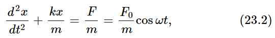
Ordinarily such a problem is very difficult because of the character and complexity of the frictional term. There are, however, many circumstances in which the frictional force is proportional to the speed with which the object moves. An example of such friction is the friction for slow motion of an object in oil or a thick liquid. There is no force when it is just standing still, but the faster it moves the faster the oil has to go past the object, and the greater is the resistance. So we shall assume that there is, in addition to the terms in (23.2), another term, a resistance force proportional to the velocity: F_f=−cdx/dt. It will be convenient, in our mathematical analysis, to write the constant c as m times γ to simplify the equation a little. This is just the same trick we use with k when we replace it by mω²₀, just to simplify the algebra. Thus our equation will be

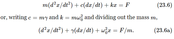
Now we have the equation in the most convenient form to solve. If γ is very small, that represents very little friction; if γ is very large, there is a tremendous amount of friction. How do we solve this new linear differential equation? Suppose that the driving force is equal to F₀ cos(ωt+Δ); we could put this into (23.6a) and try to solve it, but we shall instead solve it by our new method. Thus we write F as the real part of and x as the real part of  and substitute these into Eq. (23.6a). It is not even necessary to do the actual substituting, for we can see by inspection that the equation would become

[As a matter of fact, if we tried to solve Eq. (23.6a) by our old straightforward way, we would really appreciate the magic of the “complex” method.] If we divide by e^iωt on both sides, then we can obtain the response to the given force ; it is

Thus again is given by times a certain factor. There is no technical name for this factor, no particular letter for it, but we may call it R for discussion purposes:

(Although the letters γ and ω₀ are in very common use, this R has no particular name.) This factor R can either be written as p+iq, or as a certain magnitude ρ times e^iθ. If it is written as a certain magnitude times e^iθ, let us see what it means. Now F^=F₀e^iΔ, and the actual force F is the real part of F₀ e^iΔ e^iωt, that is, F₀ cos(ωt+Δ). Next, Eq. (23.9) tells us that is equal to R. So, writing R=ρe^iθ as another name for R, we get

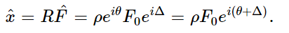
Finally, going even further back, we see that the physical x, which is the real part of the complex , is equal to the real part of ρF₀e^i(θ+Δ) e^iωt. But ρ and F₀ are real, and the real part of e^i(θ+Δ+ωt) is simply cos (ωt+Δ+θ). Thus

This tells us that the amplitude of the response is the magnitude of the force F multiplied by a certain magnification factor, ρ; this gives us the “amount” of oscillation. It also tells us, however, that x is not oscillating in phase with the force, which has the phase Δ, but is shifted by an extra amount θ. Therefore, ρ and θ represent the size of the response and the phase shift of the response.

Now let us work out what ρ is. If we have a complex number, the square of the magnitude is equal to the number times its complex conjugate; thus

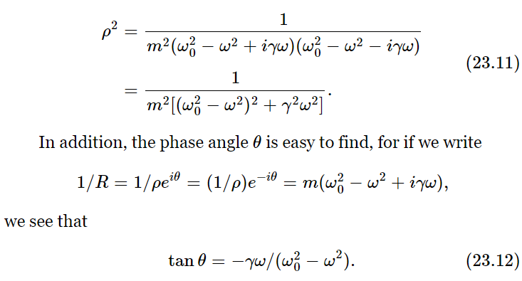
It is minus because tan(−θ)=−tan θ. A negative value for θ results for all ω, and this corresponds to the displacement x lagging the force F.

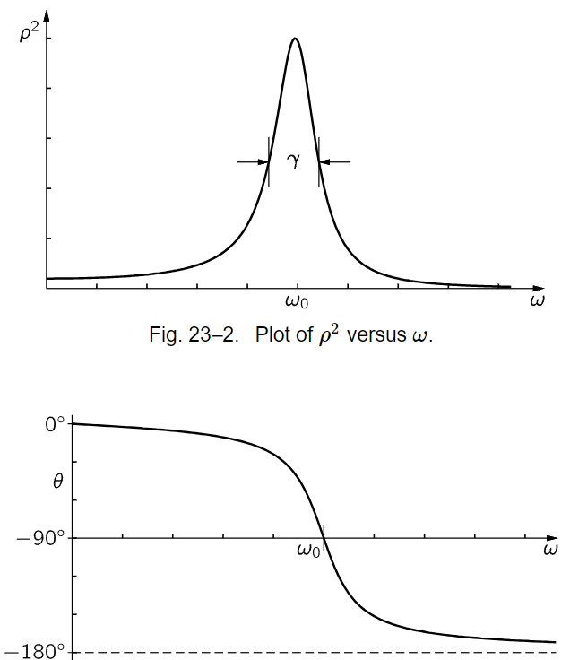
Fig. 23–3.Plot of θ versus ω.

Figure 23–2 shows how ρ² varies as a function of frequency (ρ² is physically more interesting than ρ, because ρ² is proportional to the square of the amplitude, or more or less to the energy that is developed in the oscillator by the force). We see that if γ is very small, then 1/(ω²₀−ω²)² is the most important term, and the response tries to go up toward infinity when ω equals ω₀. Now the “infinity” is not actually infinite because if ω=ω₀, then 1/γ²ω² is still there. The phase shift varies as shown in Fig. 23–3.

In certain circumstances we get a slightly different formula than (23.8), also called a “resonance” formula, and one might think that it represents a different phenomenon, but it does not. The reason is that if γ is very small the most interesting part of the curve is near ω=ω₀, and we may replace (23.8) by an approximate formula which is very accurate if γ is small and ω is near ω₀. Since ω²₀−ω²=(ω₀−ω)(ω₀+ω), if ω is near ω₀ this is nearly the same as 2ω₀(ω₀−ω) and γω is nearly the same as γω₀. Using these in (23.8), we see that ω²₀−ω²+iγω≈2ω₀(ω₀−ω+iγ/2), so that

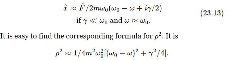
We shall leave it to the student to show the following: if we call the maximum height of the curve of ρ² vs. ω one unit, and we ask for the width Δω of the curve, at one half the maximum height, the full width at half the maximum height of the curve is Δω=γ, supposing that γ is small. The resonance is sharper and sharper as the frictional effects are made smaller and smaller.

As another measure of the width, some people use a quantity Q which is defined as Q=ω₀/γ. The narrower the resonance, the higher the Q: Q=1000 means a resonance whose width is only 1000th of the frequency scale. The Q of the resonance curve shown in Fig. 23–2 is 5.

The importance of the resonance phenomenon is that it occurs in many other circumstances, and so the rest of this chapter will describe some of these other circumstances.

مواضيع ذات صلة

The Doppler effect

Finding the “apparent” motion

Series and parallel impedances

Analogs in physics

Oscillations in linear systems

Damped oscillations

The energy of an oscillator

Complex numbers and harmonic motion

Forced oscillations

Initial conditions for Harmonic motion and circular motion

Harmonic motion and circular motion

The harmonic oscillator